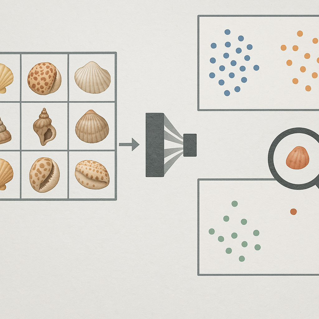
Unveiling Morphological Insights in Biological Imagery Through CNN Interpretability Techniques
Published on: 20 March 2025
Abstract
Convolutional Neural Networks (CNNs) are increasingly used in biological image analysis for tasks like species identification, but their "black box" nature
limits interpretability and trust. This study addresses this challenge by employing Explainable AI (XAI) techniques, specifically Gradient-weighted Class Activation
Mapping (Grad-CAM), to unveil the morphological insights utilized by a hierarchical CNN trained to classify species within the mollusk genus Harpa. Using a dataset
of 5837 shell images across 13 Harpa species, an EfficientNetV2B2-based model achieved high validation accuracy (96%).
Grad-CAM was applied to visualize the image
regions most influential in the CNN's classification decisions. Analysis of the resulting heatmaps revealed that the model often focuses on morphological features
consistent with traditional taxonomic descriptions, such as shoulder spines, parietal callus patterns, and body whorl coloration. However, the CNN occasionally
prioritized different features than human experts might, suggesting potential alternative diagnostic cues.
Furthermore, t-SNE visualization of the Grad-CAM heatmaps
demonstrated that the CNN employs distinct, view-dependent (apertural vs. dorsal) attention strategies for different species, with varying degrees of overlap indicating
shared visual features or potential confusion points. These findings validate the CNN's performance by linking its decisions to specific morphological characteristics,
enhance the trustworthiness of automated identification, and highlight the potential of XAI to reveal nuanced identification strategies and potentially novel biological
insights from image data.
These findings suggest new opportunities for integrating image-based learning with genetic and ecological data. Such multi-modal approaches promise to deepen our
understanding of how phenotype, genotype, and environment interact to shape biodiversity.
Introduction
The application of Convolutional Neural Networks (CNNs) has experienced a significant surge in the realm of biological image analysis. These deep learning models have demonstrated remarkable capabilities in tasks such as classifying species, detecting diseases, and segmenting various organisms, spanning the domains of botany, zoology, and marine biology [1, 3, 4]. Despite their high accuracy, the intricate internal workings of CNNs often remain opaque, functioning as "black boxes" that provide predictions without clear explanations of their decision-making processes. This lack of transparency poses a challenge, particularly in critical applications where understanding the reasoning behind a prediction is paramount for building trust and ensuring reliability [2]
To address this challenge, the field of Explainable AI (XAI) has emerged, focusing on developing techniques that can shed light on the decision-making processes of complex models like CNNs . By providing insights into why a CNN makes a particular prediction, XAI methods facilitate debugging, help identify potential biases in training data, and ultimately increase the interpretability of these powerful tools in biological research and practical applications . Among the various XAI techniques, Gradient-weighted Class Activation Mapping (Grad-CAM) [6] and saliency maps [5] have gained prominence for their ability to visualize the regions in an input image that are most influential in the CNN's output [3, 4].
Morphological features, encompassing the shape, structure, and texture of organisms, are fundamental in biological studies . These characteristics play a crucial role in species identification, disease detection, and understanding ecological relationships. Traditionally, the analysis of these features often involved manual measurements or intricate feature engineering. The advent of CNNs, coupled with interpretability techniques like Grad-CAM and saliency maps, presents an opportunity to automate and enhance the extraction and analysis of morphological features from biological images.
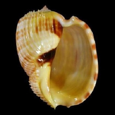
Our previously described hierarchical Convolutional Neural Network (CNN) [Hierarchical CNN to identify Mollusca], implemented within the Identifyshell.org platform, classifies Mollusca across various taxonomic levels. Within this hierarchy, the classification of the genus Harpa provides a valuable case study. Known for its unique and often intricate shell morphology, Harpa presents distinct visual features that are well-suited for demonstrating interpretability techniques like Gradient-weighted Class Activation Mapping (Grad-CAM).
In this context, Grad-CAM is employed to visualize the specific regions within shell images that contribute most significantly to the CNN's classification outcome for Harpa. Analysis of the resulting heatmaps allows for the identification of key morphological characteristics—for instance, distinct parietal callus shapes, patterns on the body whorl, or the prominence and spacing of axial ribs (varices)—that the model prioritizes. This visualization serves a dual purpose: it offers empirical validation by highlighting the features learned by the CNN, and critically, it enhances the interpretability and trustworthiness of the automated identifications provided by the system, offering potential insights into the salient diagnostic features for the genus.
Methods
Data Acquisition
Shell images were collected from many online resources, from specialized websites on shell collecting to institutes and universities. One of the largest collections of shell images is available on GBIF. Also online marketplace such as ebay contain a large collection of images. Other large shell image collections are available at , Malacopics, Femorale and Thelsica. A shell dataset created for AI is available [8].
Some online resources have facilities to download images, but most websites require a specialized webscraper. Scrapy , an open source and collaborative framework for extracting the data from websites, is used to create a custom webscraper to extract images and their scientific names. All data was stored in a MySQL database before further processing was performed.
The dataset for the Harpa CNN model comprises 5837 shell images representing 13 Harpa species (see table I). There are 14 species in the genus Harpa (WoRMS or MolluscaBase), but not enough images were found for one species. Species with less than 25 images were removed (see Minimum number of images needed for each species).
Table
| Species | # images | |
|---|---|---|
| Harpa harpa (Linnaeus, 1758) | 777 | |
| Harpa doris Röding, 1798 | 294 | |
| Harpa cabriti P. Fischer, 1860 | 747 | |
| Harpa goodwini Rehder, 1993 | 60 | |
| Harpa kolaceki T. Cossignani, 2011 | 45 | |
| Harpa davidis Röding, 1798 | 216 | |
| Harpa costata (Linnaeus, 1758) | 213 | |
| Harpa kajiyamai Habe, 1970 | 468 | |
| Harpa gracilis Broderip & G. B. Sowerby I, 1829 | 38 | |
| Harpa crenata Swainson, 1822 | 218 | |
| Harpa amouretta Röding, 1798 | 672 | |
| Harpa articularis Lamarck, 1822 | 883 | |
| Harpa major Röding, 1798 | 1228 |
Image Pre-processing
All names were checked against WoRMS or MolluscaBase for their validity. Names that were not found in WoRMS/MolluscaBase were excluded for further processing. While a large part of this data quality step was automated, a manual verification (time-consuming) step was also included. In addition to text-based quality control, both automated and manual preprocessing steps were applied to the images. Shells were detected in all images and cut out of the original image, having only 1 shell on each image. Other objects on the raw images (labels, measures, hands holding a shell, etc.) were removed. When appropiate the background was changed to a uniform black background. A square image was made by padding the black background. All shells were resized (400 x 400 px).
Model Training
For this study, Python (version 3.10.12) was used. The EffiecientNetV2B2 pre-trained models were used. (see Identifying Shells using Convolutional Neural Networks: Data Collection and Model Selection) Table 2 lists the hyperparameters. The models were trained using a batch size of 64 samples, and the number of epochs used was 50. The learning process was initiated with an initial learning rate of 0.0005 and the Adam optimiser was utilised for efficient weight updates. Two callbacks were used, one to monitor the validation loss and decreasing the learning rate , a second callback for early stopping. Both callbacks were applied to prevent the model from over-fitting. Fine-tuning the model was performed as described before. The top 30 layers of the model were unfrozen.
Table II. Hyperparameters
| Hyperparameter | Value | Comments |
|---|---|---|
| Batch Size | 64 | |
| Epochs | 50 | The number of epochs determines how many times the entire training dataset is passed through the model. Because early-stopping is used, often less than 50 epochs were needed. |
| Optimizer | Adam | The optimizer determines the algorithm used to update model weights during training. |
| Learning Rate | 0.0005 |
The validation loss was monitored and adjusted reduce_lr = keras.callbacks.ReduceLROnPlateau(monitor='val_loss', factor=0.1, patience=3, min_lr=1e-6) |
| Loss | Categorical Cross-entropy | |
| Regularization | 0.001 |
Evaluation Metrics
The evaluation of the performance of the CNN models was carried out by using standard metrics for classification: accuracy, precision, recall, and F1 score,
which are defined by [7] in terms of the number of FP (false positives); TP (true positives); TN (true negatives); and FN (false negatives) as follows:
Precision = TP/(TP + FP)
Recall = TP/(TP + FN)
F1-Score = 2 × (Precision × Recall)/(Precision + Recall)
Results
Model Training Results
The Harpa CNN model shows a good performance with a 96% validation accuracy, indicating its excellent ability to generalize to unseen data. A summary of the results of the overall model is given in table III.
Table III. Training Results
| Metrics | Value | Comments |
|---|---|---|
| Validation accuracy | 0.961 | |
| Validation loss | 0.187 | |
| Training accuracy | 0.977 | |
| Training loss | 0.141 | |
| Weighted Average Recall | 0.964 | |
| Weighted Average Precision | 0.964 | |
| Weighted Average F1 | 0.964 |
Table IV. Metrics for each species
| Species | Recall | Precision | F1 |
|---|---|---|---|
| Harpa harpa (Linnaeus, 1758) | 0.946 | 0.953 | 0.949 |
| Harpa doris Röding, 1798 | 0.968 | 0.968 | 0.968 |
| Harpa cabriti P. Fischer, 1860 | 0.924 | 0.938 | 0.931 |
| Harpa goodwini Rehder, 1993 | 0.882 | 1.000 | 0.938 |
| Harpa kolaceki T. Cossignani, 2011 | 0.857 | 1.000 | 0.923 |
| Harpa costata (Linnaeus, 1758) | 1.000 | 1.000 | 1.000 |
| Harpa kajiyamai Habe, 1970 | 0.989 | 0.989 | 0.989 |
| Harpa gracilis Broderip & G. B. Sowerby I, 1829 | 1.000 | 0.778 | 0.875 |
| Harpa crenata Swainson, 1822 | 0.961 | 0.980 | 0.970 |
| Harpa amouretta Röding, 1798 | 0.988 | 0.982 | 0.985 |
| Harpa articularis Lamarck, 1822 | 0.975 | 0.981 | 0.978 |
| Harpa major Röding, 1798 | 0.962 | 0.944 | 0.953 |
Some species with fewer training examples exhibited more variability. For instance, Harpa gracilis (recall: 100%, precision: 77.8%, F1: 87.5%), despite high recall, showed lower precision, suggesting challenges in avoiding false positives, likely due to the limited number of images. Conversely, Harpa goodwini (recall: 88.2%, precision: 100%, F1: 93.8%) and Harpa kolaceki (recall: 85.7%, precision: 100%, F1: 92.3%) had perfect precision but slightly lower recall, indicating the model was cautious but occasionally missed identifying these species correctly, possibly reflecting limited training data.
Other species demonstrated balanced and robust results, such as Harpa doris (recall, precision, and F1 each at 96.8%), Harpa crenata (recall: 96.1%, precision: 98.0%, F1: 97.0%), and Harpa amouretta (recall: 98.8%, precision: 98.2%, F1: 98.5%), showing strong overall classification capabilities. The moderate performance observed for Harpa cabriti (recall: 92.4%, precision: 93.8%, F1: 93.1%) and Harpa harpa (recall: 94.6%, precision: 95.3%, F1: 94.9%) indicated stable yet slightly less precise results, even with ample training data.
Overall, the Harpa CNN model effectively captured distinguishing characteristics for each species, demonstrating robust predictive performance while showing slight variability influenced by the distinctiveness of features and, to some extent, the number of training samples available per species.
Confusion matrix
The confusion matrix, shown in figure 1, confirms the strong overall performance of the Harpa CNN model, while highlighting specific areas of confusion among certain species. The matrix clearly illustrates high accuracy along the diagonal, indicating correct classifications, consistent with previously reported precision, recall, and F1 scores.
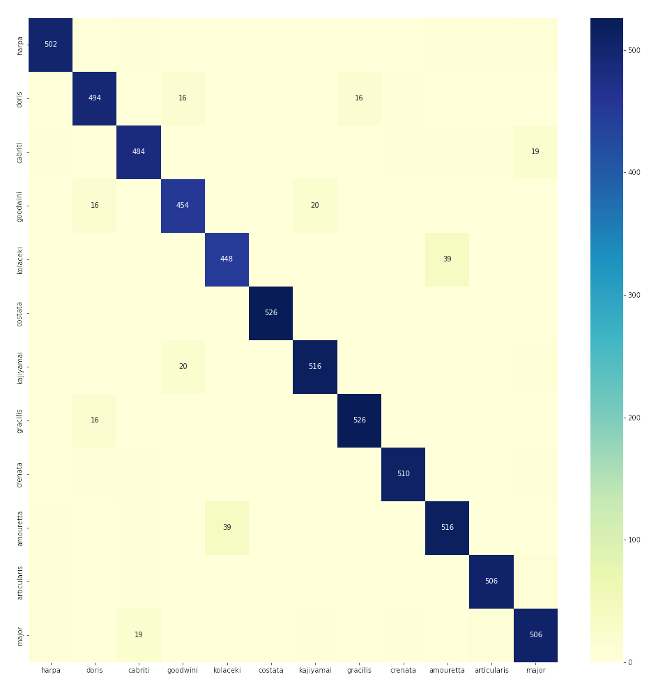
Figure 1: Confusion matrix
However, some notable confusions are present. A small number of images from Harpa kolaceki and Harpa goodwini, both species with fewer training examples, are incorrectly classified, confirming the previously described lower recall for these species. Similarly, the confusion matrix reveals why Harpa gracilis exhibited lower precision—despite high recall—with several instances from other classes incorrectly predicted as gracilis.
Misclassifications primarily occur between visually similar species or species with limited training images. For example, a few images of Harpa cabriti and Harpa harpa, both species with relatively large datasets, were occasionally confused, indicating visual similarities challenging the CNN model’s discrimination capabilities.
Overall, the confusion matrix supports earlier findings, highlighting strong accuracy across most classes while clarifying specific areas of minor confusion, typically among visually similar species or species with fewer training examples.
Note that Harpa davidis is not used for training despite sufficient images available. This species was removed because it was often confused with Harpa major. More than 20% of all Harpa davidis was confused with Harpa major (and vice versa).
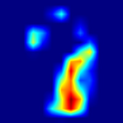
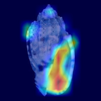
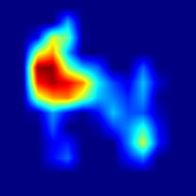
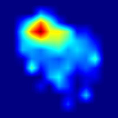
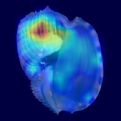
Grad-CAM
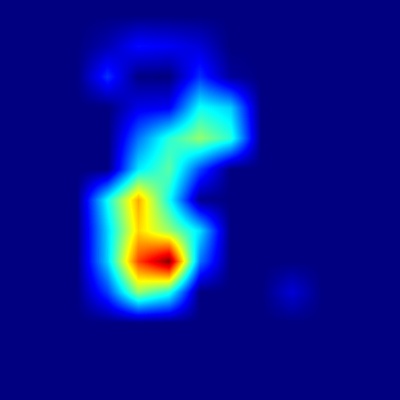
A GRAD-CAM visualisation technique was used to understand the prediction process and emphasise the intriguing areas of the shell pictures that
determine the final decision.The visual explanation provides an overview by generating a heatmap where pixels with high to low intensity are indicated
in red, yellow, green and blue [6]. This technique can be used to determine whether the model accurately predicts the species.
A few typical examples are given in figure 2.
Figure 2: Typical examples of a heatmaps generated with Grad-CAM
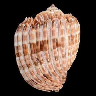
| Species | Original Image | Heatmap | Superimposed image |
|---|---|---|---|
|
Harpa amouretta Röding, 1798 Apertural view |
 |
 |
 |
|
Harpa articularis Lamarck, 1822 Apertural view |
 |
 |
 |
|
Harpa cabriti P. Fischer, 1860 Apertural view |
 |
 |
 |
|
Harpa costata (Linnaeus, 1758) Apertural view |
 |
 |
 |
|
Harpa costata (Linnaeus, 1758) Dorsal view |
 |
 |
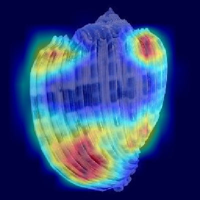 |
Grad-CAM
For each species and viewpoint (apertural and dorsal views), average heatmaps were generated to visualize regions most influential for the CNN model's species identification.
Each visualization consists of two images: the left image displays the heatmap intensity alone, clearly indicating activation patterns. The right image overlays this heatmap
onto an actual shell image of the corresponding species and viewpoint. In these visualizations, areas highlighted in red or orange represent regions with the highest activation
by the CNN model, meaning these specific areas of the shell contain the critical features the model uses to distinguish between species. In the following section, we provide
detailed descriptions of these heatmaps for each species, discussing how the activated regions align with diagnostic features described in the literature for accurate identification
of Harpa species.
Harpa amouretta
.png)
Figure 3: Harpa amouretta - Apertural view
.png)
Figure 4: Harpa amouretta - Dorsal view
Based on the Grad-CAM visualizations, the Convolutional Neural Network appears to utilize distinct morphological features of Harpa amouretta depending
on the perspective presented. When analyzing the apertural view, the model shows strong activation concentrated on the lower portion of the shell, particularly
around the columellar area and the siphonal notch. This focus aligns remarkably well with the description's emphasis on the characteristic chestnut blotches
found on the inner lip – specifically the central blotch near the parietal/columellar juncture and the basal blotch near the anterior canal – which are key
diagnostic features for this species.
Conversely, when presented with the dorsal view, the heatmap indicates that the CNN directs its attention primarily to the flank of the shell, with high
activation along the left side covering the body whorl and extending partially onto the lower spire.
This dorsal focus strongly suggests the model is
leveraging the distinctive surface details described for H. amouretta [8]. The most likely features driving this activation are the complex color patterns,
such as the festooned or zigzag chestnut markings within the intercostal spaces, as well as the numerous fine, paired chestnut lines decorating the axial ribs
themselves. Additionally, the structural characteristics of the ribs and the shoulder angulation in this highly activated region might also contribute to the
model's identification process from this perspective.
In essence, the CNN effectively identifies Harpa amouretta by focusing on different but equally significant diagnostic traits highlighted in its
morphological description: the unique ventral blotches visible from the front, and the intricate color patterns and rib structures prominent
on its dorsal flank.
Harpa articularis
.png)
Figure 5: Harpa articularis - Apertural view
.png)
Figure 6: Harpa articularis - Dorsal view
An important diagnostic feature for Harpa articularis is that the entire columnella is typically covered by a large, dark blotch, as documented
in the literature [8]. Examining the heatmaps generated for this species reveals insights into how the CNN model aligns with known
identification criteria.
When examining the apertural perspective, the model demonstrates strong activation concentrated primarily on the upper portion of the shell, encompassing the spire
and the critical shoulder area of the body whorl. This focus aligns well with the described morphological complexities in this region, particularly the strong,
angular denticulation of the ribs at the shoulder and the potential presence of a shallow groove just below it. Intriguingly, the heatmap shows minimal activation
over the lower ventral surface, indicating that the large, uninterrupted chestnut-colored splotch covering the parietal and columellar calluses – a key diagnostic
feature for human observers – is not the primary focus for the CNN in this view.
In contrast, the dorsal view heatmap
highlights the overall shell shape as influential in recognizing this species, with the highest activation specifically concentrated near the basal
portion of the outer lip. This indicates that the CNN utilizes both detailed anatomical features, such as distinctive coloration patterns, as well as
overall morphological characteristics to reliably identify H. articularis.
The crucial difference in how the model identifies H. amouretta and H. articularis lies in the type and location of features it prioritizes. Harpa amouretta is recognized primarily through its distinctive color patterns, with the CNN focusing on the apertural blotches situated low on the shell and the intricate patterns decorating its mid-dorsal flank. Conversely, the identification of Harpa articularis appears driven more by structural features; the model concentrates on the shoulder complexity high on the aperture and the shell's form at the dorsal base and shoulder, while notably overlooking the species' major ventral color patch. This divergence indicates the CNN has learned to differentiate them by prioritizing different kinds of visual cues – leveraging prominent color patterns for amouretta and specific structural shapes and details for articularis.
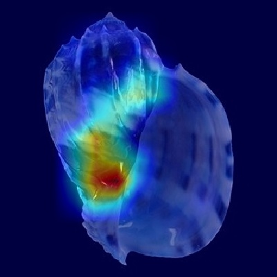
Harpa cabriti
.png)
Figure 7: Harpa cabriti - Apertural view
.png)
Figure 8: Harpa cabriti - Dorsal view
The Grad-CAM heatmaps for Harpa cabriti correspond closely with the key shell characteristics detailed in the provided species description, indicating
the Convolutional Neural Network leverages biologically significant features for identification. According to the description [8, 9],
defining traits include prominent ribs bearing distinct lamellar projections, particularly at the shoulder, and characteristic color patterns involving blotches,
bands, and festoon-like lines.
Examining the apertural view, the heatmap shows strong activation concentrated around the upper portion of the body whorl, near the junction with the outer lip.
This region accurately encompasses the location of the strong, spinose projection on the ribs at the shoulder and also coincides precisely with the position of
the large upper chestnut spot described on the parietal wall. This alignment reinforces that the model recognizes both the crucial structural detail of the
shoulder spine and the specific color marking near the aperture's top as vital identifiers from this perspective.
Similarly, the dorsal view heatmap displays pronounced activation across the central upper body whorl and shoulder region, highlighting the ribs and the
intervening spaces. This focus corresponds directly with the described sculptural and color features visible from the back: specifically, the ribs bearing
their lamellar, spinose projections at the shoulder and the distinctive dorsal color scheme, including the revolving bands created by alternating blotches
and white stripes on the ribs and the festoonlike chestnut markings within the interspaces.
Overall, the CNN's activated regions in both views align strongly with Harpa cabriti's described morphological and color features, particularly the structurally
complex and pattern-rich shoulder area. This demonstrates that the model effectively identifies the species by focusing on a combination of biologically
meaningful characteristics, namely the shoulder spines and view-specific color patterns.
Harpa costata
.png)
Figure 9: Harpa costata - Apertural view
.png)
Figure 10: Harpa costata - Dorsal view
In the apertural view heatmap, the strongest activations appear on the upper portion of the body whorl, especially around the shoulder angle and adjacent regions.
This precisely matches the shell description, which highlights distinctive ribs with triangular, spine-like projections at the shoulder forming a subsutural channel.
The heatmap confirms that the model strongly relies on these prominent ribs and projections to distinguish H. costata.
Similarly, the dorsal view heatmap strongly emphasizes the ribs across the central and peripheral body whorl areas, consistent with the shell description
mentioning numerous crowded, lamellar ribs with distinct spine-like projections. Additionally, the activated regions correspond closely to the described
coloration patterns, such as chestnut spots and bands of varying darker shades between the ribs, confirming that these color and rib patterns together
provide critical identification cues for the CNN model.
Overall, the visual examination of both heatmaps confirms strong alignment with the morphological and color features detailed in the shell's
literature description [8], providing clear visual evidence that the CNN model uses biologically meaningful and well-defined shell
characteristics to identify Harpa costata.
Harpa crenata
.png)
Figure 11: Harpa crenata - Apertural view
.png)
Figure 12: Harpa crenata - Dorsal view
Comparing the provided shell description of Harpa crenata with the visual heatmaps reveals a clear correspondence between morphological
characteristics detailed in the literature and the regions activated by the CNN model.
In the apertural view heatmap, significant activation occurs mainly along the left side of the body whorl. This region corresponds to the
pronounced curvature and the external color pattern described in the literature, including axial chestnut markings and distinctive coloration
between the ribs [8]. Thus, the CNN strongly relies on these visual and color features present on the left side of the shell
for accurate species identification.
In the dorsal view heatmap, strong activation is observed prominently at the shoulder and basal portions of the body whorl. These activated areas
directly match the shell description highlighting an angulated shoulder with triangular, lamellar spines and characteristic basal curvature.
The pronounced activation on these morphological features suggests that the CNN effectively identifies H. crenata by detecting the distinctive
spines, ribs, and shape described in the literature.
Overall, this corrected analysis clearly confirms the alignment between the CNN model’s activated heatmap regions and key morphological and
coloration features described for Harpa crenata, indicating the model's reliance on biologically meaningful shell traits for species identification.
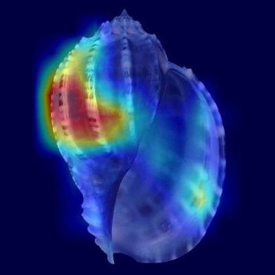
Harpa doris
.png)
Figure 13: Harpa doris - Apertural view
.png)
Figure 14: Harpa doris - Dorsal view
Comparing the provided shell description of Harpa doris with the visual heatmaps reveals a strong correspondence between the described morphological
characteristics and the activated regions identified by the CNN.
The apertural view heatmap demonstrates strong activation on the left side of the body whorl, opposite the aperture, closely aligning with the shell's described
features. The description emphasizes distinct ribs marked by brown interrupted lines, narrow bands with chestnut markings, and characteristic bicolored bands
consisting of orange and purplish-pink blotches, all predominantly visible along this region. These visual and color features are therefore clearly crucial
cues used by the CNN model for accurate species identification.
In the dorsal view heatmap, activation occurs strongly along the left side of the shell, corresponding to the position of the outer lip when viewed dorsally.
This activated region closely matches the literature description, particularly the presence of prominent triangular spines at the shoulder angulation and
distinct rib patterns. These structural features along the outer lip region, as described, seem to strongly inform the CNN's identification decisions.
Harpa harpa
.png)
Figure 15: Harpa harpa - Apertural view
.png)
Figure 16: Harpa harpa - Dorsal view
The visual heatmaps for Harpa harpa strongly align with the described morphological and coloration features of this species. In the apertural view heatmap,
significant activation occurs prominently at the spire and shoulder region of the body whorl. This corresponds precisely with the literature description emphasizing
the stout, broadly ovate shell shape with a notably flattened subsutural ramp and distinct angulation marked by strong spines at the shoulder of the body whorl.
Additionally, a secondary activation near the columellar region corresponds well with the described presence of distinct reddish-brown blotches on the ventral
side and around the columellar lip, suggesting the CNN effectively utilizes these color patterns for species recognition.
In the dorsal view heatmap, high activation is observed at two important areas: the shoulder of the body whorl and the basal region near the outer lip.
The activation at the shoulder closely matches the shell description emphasizing strong, flattened ribs crossed by distinctive fine dark lines grouped together.
The activated basal area corresponds clearly to described patterns of reddish-brown blotches, wavy axial stripes, and spiral bands with chestnut
spots—features that collectively represent key visual cues for the CNN.
Overall, both heatmaps indicate that the CNN model's identification process for Harpa harpa strongly relies on biologically relevant, visually distinct shell
features described in the literature, particularly the pronounced shoulder structure, distinctive ribs, and characteristic coloration patterns.
Harpa kajiyamai
.png)
Figure 17: Harpa kajiyamai - Apertural view
.png)
Figure 18: Harpa kajiyamai - Dorsal view
Comparing the provided shell description of Harpa kajiyamai with the visual heatmaps demonstrates a clear correspondence between the literature and
the CNN activations.
The apertural heatmap shows strong activation primarily on the left side of the body whorl. This activated region aligns closely with the literature's
description highlighting the presence of distinctive coloration patterns, including bands with dark lines grouped in pairs or triplets, and the
conspicuous ribs sharply angled at the shoulder. This suggests that the CNN model accurately identifies the species using these rib features and
distinct color patterns on the external surface of the body whorl.
In the dorsal heatmap, activation prominently occurs on the left side, corresponding clearly with the outer lip region in dorsal orientation.
This activation strongly matches features emphasized in the description, including the sharply acuminate ribs at the shoulder, their flattened
reflections near the base, and distinctive spiral banding coloration patterns. The strong activation along the dorsal side's outer lip confirms
that the CNN recognizes and relies upon these well-described morphological and coloration features for accurate identification.
The CNN heatmaps align closely with the defining morphological and coloration features documented for Harpa kajiyamai,
indicating the model’s reliance on biologically significant and visually distinctive shell traits described explicitly in literature [8].
Harpa major
.png)
Figure 19: Harpa major - Apertural view
.png)
Figure 20: Harpa major - Dorsal view
Comparing the provided shell description of Harpa major with the visual heatmaps reveals a strong correspondence between the CNN model’s activated regions
and the key features described in literature, with some interesting details worth noting.
In the apertural view heatmap, significant activation occurs in two distinct regions: the center of the body whorl and along the middle of the outer lip.
This aligns closely with the literature’s emphasis on prominent ribs and their characteristic coloration, including variable chestnut lines and the notable,
centrally divided chestnut blotch covering the parietal wall. The centrally activated region corresponds particularly well with the described chestnut blotch
pattern, a key diagnostic characteristic for identifying this species.
In the dorsal view heatmap, activation is most prominent on the right side, corresponding to the body whorl curvature and strongly emphasizing the broad,
heavy ribs described as distinctly angulated at the shoulder and contributing to the characteristic shell outline. Additionally, activation on the left side,
corresponding to the dorsal side of the outer lip, aligns well with described color patterns and the structural outline of the shell’s aperture.
Thus, the CNN model clearly utilizes both the ribs' structural prominence and their associated color patterns for identification.
Visualization of identification strategies used for each species
Based on our analysis of the average Grad-CAM heatmaps, we characterized the dominant visual strategy the CNN employs to identify each Harpa species studied. It became clear that the model utilizes distinct approaches for different species, rather than relying on a single, uniform strategy across the genus. A significant variation observed lies in the type of features prioritized by the network; in some instances, color patterns appear paramount for identification, while for other species, aspects of the shell's structure command more of the model's attention. For example, recognizing Harpa amouretta seemed strongly linked to its specific color patterns, such as apertural blotches and dorsal markings. Conversely, identifying Harpa articularis and Harpa cabriti involved a greater focus on structural features, particularly the complexities of the shoulder region, although specific color cues clearly contributed to the strategy for H. cabriti as well.
To visualize these different strategies we have used t-SNE [12].
t-SNE is a visualization technique to help understand the different attention strategies of the Harpa CNN model uses
for each Harpa species, based on their Grad-CAM heatmaps. It converts the heatmap data into a 2D plane while attempting to keep similar heatmap patterns close together.
Each species and view is colour coded to allow to see the different strategies used for each species.
Distinct separation between different colored groups visually confirms that the model employs different attention patterns for those respective species. Conversely, areas where
different colors mix and overlap highlight instances where similar visual strategies were used across species, potentially indicating shared features or sources of confusion
for the model.
Furthermore, this visualization can reveal variations within a single species. If points representing a single species, indicated by a single color, form multiple distinct
clumps within the plot, this provides strong visual evidence that the model utilizes alternative strategies to identify even that one species across different images.
The density and spread of points for each color also offer insights into the consistency or variability of the strategy used for each species. In essence, t-SNE provides a
visual map of the model's learned attention patterns, allowing you to explore how identification strategies compare across species and whether diverse strategies exist within them.
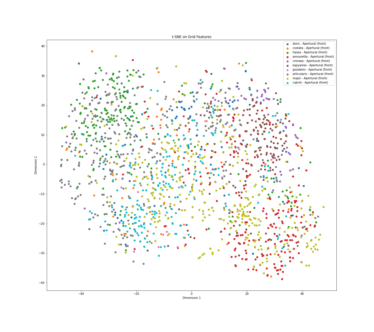
Figure 21: t-SNE Visualization of 10 Harpa species heatmaps - Apertural view
This t-SNE visualization maps the similarities between Grad-CAM heatmaps generated from apertural views of ten different Harpa species, with each point colored according to its true species label. The plot reveals an underlying structure rather than random scatter, indicating that the model's attention patterns have detectable similarities and differences. However, while there are visible grouping tendencies, the visualization is also characterized by significant overlap and mixing between the colors representing many species, alongside noticeable variability within individual species categories.
Several species demonstrate relatively unique attention patterns. Harpa articularis, represented by Yellow/Olive points, forms a cohesive cluster in the bottom right, suggesting a distinct strategy. Harpa cabriti, shown as Grey points, also groups effectively in the middle-right, indicating a fairly unique focus. To a lesser extent, Harpa kajiyamai (Brown) shows clustering tendencies in the middle-right, suggesting some distinction in the strategy.
Conversely, there is substantial mixing in the left and central parts of the plot. Harpa major, represented here by Cyan / Light Blue points, is widely distributed and
heavily overlaps with Harpa doris (Blue), Harpa costata (Orange), Harpa harpa (Green), Harpa amouretta (Red), and Harpa crenata (Purple). This indicates that the visual
attention patterns used for H. major share significant similarities with those used for these other species in the apertural view. Harpa amouretta (Red) and Harpa crenata
(Purple) are particularly mixed within this larger group on the left side.
This extensive overlap suggests that the attentional strategies employed by the model for these particular species share significant visual
similarities when viewed from the aperture, potentially indicating shared important features or areas where the model might find differentiation challenging.
Furthermore, the spread observed for most species suggests considerable intra-species variation in the model's focus across different images.
In summary, this t-SNE analysis visually confirms that while the CNN has learned distinct apertural attention patterns for species like Harpa articularis and Harpa cabriti, the strategies used for many other species appear less differentiated and show considerable resemblance to one another, particularly centering around the patterns associated with Harpa major.
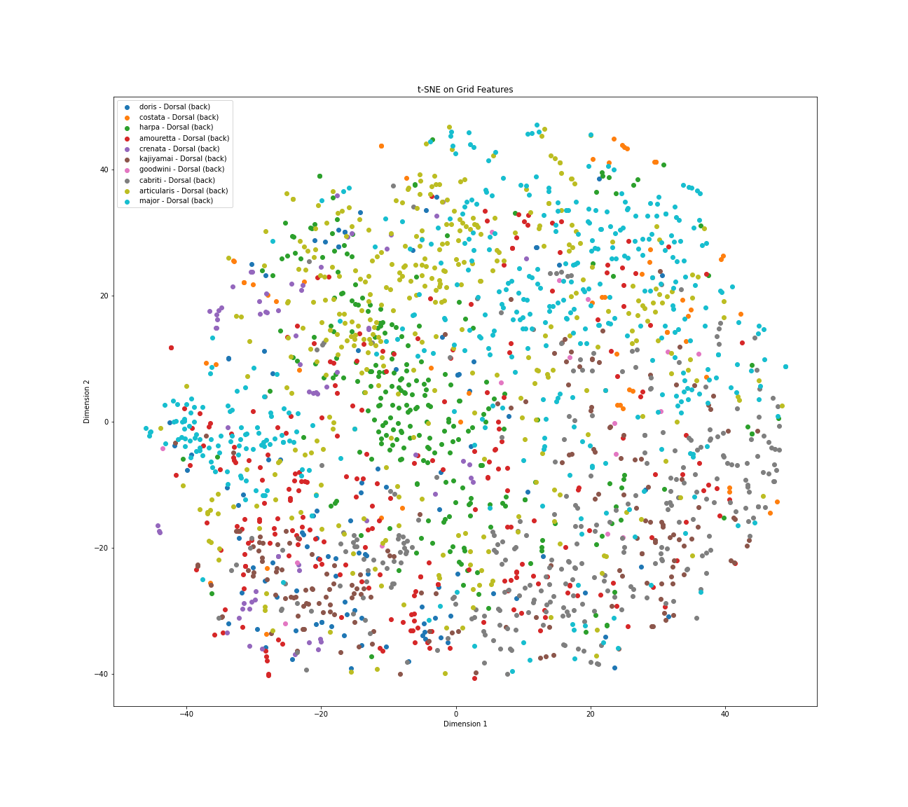
Figure 22: t-SNE Visualization of 10 Harpa species heatmaps - Dorsal view
Analyzing the t-SNE visualization generated from the dorsal view Grad-CAM heatmaps for the ten Harpa species provides further insights into the model's identification strategies. As with the apertural view, this plot shows inherent structure with points grouped based on heatmap similarities, yet significant overlap between species' attention patterns persists. Notably, the overall arrangement and relative positioning of the species clusters differ distinctly from the apertural view map, confirming that the model generally employs different visual approaches depending on whether it sees the front or the back of the shell.
Several species appear to utilize relatively distinct dorsal attention strategies. Harpa articularis, represented by Yellow/Olive points, forms a cohesive cluster in the lower-left quadrant, suggesting a unique dorsal focus. Similarly, Harpa cabriti, shown as Grey points, groups reasonably well in the bottom-center area, indicating a distinct strategy. In the upper right, Harpa kajiyamai (Brown) also forms relatively separated cluster. Additionally, Harpa crenata (Purple) shows a clear tendency to cluster in the lower left.
However, significant overlap persists in the central and upper-left regions. Harpa major, now represented by Cyan/Light Blue points, remains widely distributed throughout these areas, intermingling heavily with Harpa costata (Orange), Harpa harpa (Green), and Harpa doris (Blue). This indicates substantial visual similarity between the dorsal attention patterns used for H. major and these other species. In the lower left, Harpa amouretta (Red) points are concentrated near and appear to overlap with Harpa crenata (Purple).
In conclusion, the dorsal view t-SNE analysis reveals that while some species like H. articularis and H. cabriti utilize distinct attention strategies irrespective of view, many species exhibit dorsal heatmap patterns that are visually similar to each other, especially clustering around the varied patterns used for H. major. These relationships and overlaps differ from those observed in the apertural view, highlighting the view-dependent nature of the model's learned visual strategies for identifying these Harpa shells.
Discussion
The results show that a convolutional neural network (CNN) trained on mollusk shell images is able to identify different species using features that often align with those used by human experts, such as shoulder spines, parietal spots, and distinct color patterns. Grad-CAM visualizations confirm that the network’s attention focuses on these regions, addressing concerns about the “black box” nature of deep learning and suggesting that the features uncovered by the CNN may also possess phylogenetic relevance. Interestingly, in some cases, the CNN ignored or de-emphasized traits that taxonomists consider critical, such as the ventral blotch in H. articularis. This might indicate that the model identifies equally valid or more consistent cues across varying photographic conditions, potentially yielding new insights into shell morphology. This observation was also made in others studies on plants [10] and fish [11].
The model achieved high overall accuracy (96% validation), indicating robust generalization. Species-specific performance was generally strong, particularly for species with distinct features and adequate data like H. costata (perfect metrics) and H. kajiyamai (98.9% F1). Grad-CAM analysis revealed the model's focus aligns well with diagnostic characteristics across multiple species.
Species-specific patterns highlight the diversity of strategies the CNN adopts. For example, H. amouretta tends to be classified through bold color banding, while H. articularis is often separated by rib structures and shoulder spines. H. cabriti appears to prompt a blend of approaches—some focus on color, others on form. Smaller classes, like H. gracilis, H. goodwini, and H. kolaceki, suffered from limited sample sizes, leading to more confusion in the model outputs. t-SNE plots reinforced these observations by showing distinct clusters for certain species, yet overlapping distributions for those with subtle morphological differences or within-species variation, particularly in H. major. The correlation between high accuracy scores and clear Grad-CAM focus suggests the CNN’s learned features are genuinely informative, whereas persistent misclassifications — like cabriti/harpa — likely reflect genuine visual similarities.
These findings underline the broader importance of explainable AI (XAI) methods in biological morphology. By localizing important regions in shell images and mapping them to known taxonomic features, Grad-CAM and t-SNE strengthen trust in automatic identification tools while revealing possible alternative diagnostic cues. Integrating genotype and environmental data offers an avenue for even deeper inquiry into how morphological traits develop in response to genetic lineage and ecological conditions, thus bridging phenotype, genotype, and environment within a single analytical framework [13]. This could uncover how inheritance and adaptation shape species’ shell appearances.
Crucially, these observations point to the prospect of deeper biological insights when other data modalities—especially genotype and environment—are integrated. In other domains, CNNs have successfully fused morphological images with genetic and ecological datasets [14], revealing how phenotypic variation can be attributed to lineage-specific genetic factors or localized environmental pressures. Adapting this multi-modal framework to mollusks could yield a more holistic account of how heritable traits and environmental conditions converge to shape shell form [15]. For example, aligning CNN-extracted features with DNA barcoding data might help confirm (or discover) cryptic species [14] and clarify the evolutionary significance of morphological traits. Likewise, incorporating habitat variables would enable exploration of adaptive shell variations—such as the potential role of substrate, temperature, or predation levels in influencing color patterns or shell thickness.
Despite these promising results, certain limitations remain. Web-scraped images can contain labeling errors or exhibit wide variability in lighting and angle. Rare species are underrepresented, affecting classification accuracy and interpretability. Methods like Grad-CAM, though illuminating, show only where the model is focusing, not the complete causal reasoning behind its decisions. Parameter sensitivity in t-SNE and the challenge of interpreting three-dimensional shells from two-dimensional photos further constrain the depth of these analyses. Interpretations of localized heatmaps also depend on expert opinion, underscoring the subjectivity inherent in mapping network activations to named morphological traits.
Looking ahead, a priority is to incorporate genetic markers or ecological metadata to better contextualize the anatomical features identified by CNNs. By coupling shell images with data on habitat conditions and genotypic variation, it becomes possible to explore how environment and lineage shape phenotype. Additional XAI approaches, such as LIME or SHAP, could provide more nuanced explanations, while more systematic clustering of heatmaps might uncover hidden identification “strategies” within or across species. Addressing misclassifications by scrutinizing Grad-CAM outputs in incorrect predictions could refine data collection strategies and clarify whether confusions stem from genuine morphological overlaps or overlooked diagnostic features. These extensions, along with user-oriented evaluations of how well these visual explanations enhance trust, hold promise for advancing automated shell identification and for fostering richer insights into the evolutionary processes that sculpt morphological diversity.
References
- [1] Meraj T. et al. Computer vision-based plants phenotyping: A comprehensive survey. iScience. 12;27(1):108709 (2023)
- [2] Mkhatshwa, J. et al. Analysing the Performance and Interpretability of CNN-Based Architectures for Plant Nutrient Deficiency Identification. Computation 12, 113. (2024)
- [3] Yi-Chin Lu, et al. Identifying the species of harvested tuna and billfish using deep convolutional neural networks. ICES Journal of Marine Science, Volume 77, Issue 4, Pages 1318–1329 (2020)
- [4]S. Kiel Assessing bivalve phylogeny using Deep Learning and Computer Vision approaches bioRxiv 2021.04.08.438943 (2021).
- [5] Simonyan, K. et al. Deep Inside Convolutional Networks: Visualising Image Classification Models and Saliency Maps. arXiv:1312.6034. (2013)
- [6] Selvaraju, R et al. Grad-CAM: Visual Explanations from Deep Networks via Gradient-based Localization. arXiv:1610.02391 (2016)
- [7] Powers, D. M. W. Evaluation: From Precision, Recall and F-measure to ROC, Informedness, Markedness & Correlation. Journal of Machine Learning Technologies, 2(1), 37–63. (2011)
- [8] Rehder H.A. The family Harpidae of the world. Indo-Pacific Mollusca 3(16) : 207-274 (1973)
- [9] Okon, M.E. The Genus Harpa Revisited. American Conchologist Volume 32 (3), 4-13 (2004)
- [10] P. Wilf et al. Computer vision cracks the leaf code. Proc. Natl. Acad. Sci. U.S.A., 113 (12) , 3305–3310 (2016)
- [11] Elhamod, M. et al. Hierarchy-guided neural network for species classification. Methods in Ecology and Evolution, 13, 642–652 (2022)
- [12] van der Maaten, L., & Hinton, G. Visualizing Data using t-SNE.. Journal of Machine Learning Research, 9(Nov), 2579–2605. (2008)
- [13] Yang, B. et al. Integrating Deep Learning Derived Morphological Traits and Molecular Data for Species Identification. Systematic Biology, 71(3), 690–705 (2022)
- [14] Badirli, S. et al. Classifying the unknown: Insect identification with deep hierarchical Bayesian learning. Methods in Ecology and Evolution, 14(6), 1515–1530 (2023)
- [15] Concepción, R. et al. BivalveNet: A hybrid deep neural network for common cockle geographical traceability based on shell image analysis. Ecological Informatics, 78, 102344 (2023)