Coping with the open-world problem when identifying Mollusca
Published on: January 26, 2025
Abstract
The open-world problem in species identification using Convolutional Neural Networks (CNNs) arises when the models encounter classes or data distributions beyond their training scope, leading to misclassifications and error propagation in the hierarchical CNN setup. In this paper, we examine the open-world problem in the context of Mollusca shell identification, where a hierarchical CNN is used to first identify the order, then the family, and finally the genus and species. Addressing this challenge involves integrating OOD detection into hierarchical CNNs. By recognizing and rejecting unseen classes early in the classification process, OOD detection minimizes cascading errors and provides reliable outputs at higher taxonomic levels. Techniques such as outlier detection, anomaly detection, and confidence-based thresholds are explored to enhance the robustness of hierarchical models. While the inclusion of OOD detection slightly reduces performance metrics like F1 scores, it improves the system's ability to manage real-world complexity and adapt to images of unknown species, thereby enhancing its applicability in species classification tasks.
Introduction
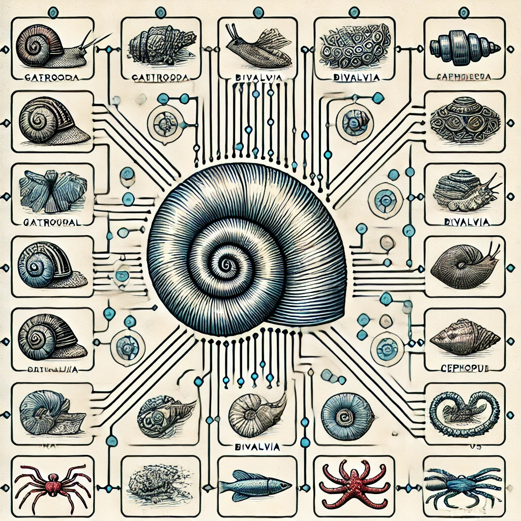
The open-world problem in the context of Convolutional Neural Networks (CNNs) (or AI models in general) refers to challenges that arise when these models encounter situations, classes, or data distributions they were not explicitly trained on. Unlike closed-world scenarios, where the system is only expected to operate within a predefined and limited set of classes or conditions, open-world problems require the system to adapt, generalize, or handle unseen data effectively. A CNN is designed to work in a closed-world situation, it does not expect to see images of classes outside the ones it is trained [6]. Because we have not included all species in our models to recognize Mollusca, we are in an open-world situation. To illustrate, see Figure 1, where we trained a family, Cymatiidae, on many genera that belong to the same family. A good model that knows the 6 genera seen during training will classify new images (shown at the left) in one of the 6 genera. However, when one of the images to right are presented to the model - that does not belong to one of the 6 genera - it will still categorize it in one of the known genera, while the images shown to the right in the image below belong to a completely different family. Moreover, it might identify them to belong to one of the 6 genera with high confidence [13]. This will also occur when an image is presented of a species that belong to another genus of the same family for which the model was not trained.
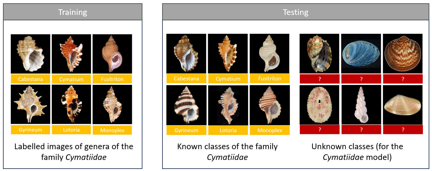
Figure 1: The model identifies images within the 6 genera it was trained on but fails with OOD images, misclassifying them into known genera.
Open-world learning provides a framework in which CNNs can not only classify known objects but also flag unknown inputs and adapt accordingly. This ability is vital for real-world applications such as species recognition, where new species are routinely discovered. In the context of biological classification tasks like recognizing species within the phylum Mollusca, a model trained on a limited subset of known species will inevitably encounter previously unobserved ones. Note that we need a minimum number of images per species before we can include the species in the training image dataset. Addressing this challenge demands that the CNN go beyond mere classification, embracing open-world learning principles to adapt and generalize effectively. In this article, we explore strategies and approaches that enable CNNs to thrive in open-world environments. We discuss the challenges posed by new species, variations in environmental conditions, and limited training data.
An open-world classification CNN should be able (1) to assign images to one of its trained classes or else reject the images (unseen classes), (2) discover unseen classes in the rejected examples and (3) update the CNN with new classes [1]. In this article we focus on the first capability; rejecting unseen classes. Open-world classification is also known as out-of-distribution (OOD) detection. Two types of images can be OOD: (1) an image with a species that belongs to one of the classes on which the model was trained, but the image shows the species from an unusual viewpoint, or with unseen colours, contrast or brightness or (2) images of new species, or species on which the model was not trained (also called out-of domain images) [4], [5]. There are several approaches to OOD detection. These include outlier detection [7], anomaly detection [8], novelty detection [9], and open set recognition [10]. Some approaches are more suitable to one of the 3 desired capabilities mentioned before.
Outlier detection
In this approach, the CNN model is trained on outliers too, not only the set of in-distribution classes or species. One of the core strengths of outlier detection (OE) lies in how it explicitly teaches the model about data it should not recognize. Traditional CNN training focuses solely on the in-distribution classes—e.g., dog vs. cat classification — without any explicit “negative examples.” By contrast, OE broadens the learning process to include representative samples from unrelated distributions. Consequently, the CNN learns a more discriminative boundary between in-distribution data and everything else, leading to better OOD detection capabilities [16]. To illustrate see figure 2, where we have the same classes to train as depicted in figure 1, but this time we add during training images that are out-of-distribution for the model. During the test phase, we will check if the OOD images belong to the OOD class. The new model is able to identify other images of shells that belong to one of the 6 genera, but also able to identify 'unknown' classes.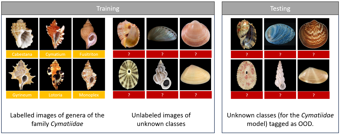
Figure 2: Adding an OOD class during training allows the model to identify and separate unknown species.
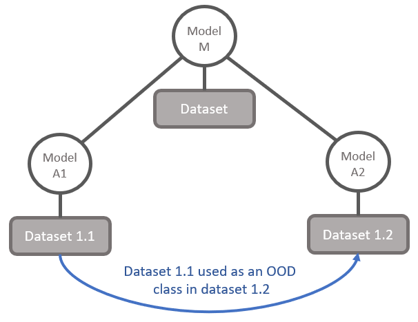
Figure 3: Using the images of the dataset used for one model as an OOD class in the dataset of another model on the same taxonomic level (e.g. family).
For example, for all 'family' models that are trained on images that belong to a particular family, we will add an OOD class that contains a sample of images from the other families.
OOD detection using thresholds
The approaches for OOD detection span confidence-based methods, probabilistic models, feature analysis, and ensemble techniques, among others. Confidence-based methods are among the simplest strategies for OOD detection, relying on the model's prediction confidence to identify OOD images. For instance, softmax confidence thresholding assumes that OOD samples tend to have lower softmax probabilities than in-distribution samples. When the maximum softmax probability of a sample falls below a predefined threshold, the sample is flagged as OOD [11]. Despite its simplicity, this method has limitations, particularly when the model produces overconfident predictions for OOD inputs [13]. A more refined approach, temperature scaling, adjusts the logits before applying the softmax function. This spreads the softmax distribution, improving the calibration of confidence scores and enhancing OOD detection. However, temperature scaling requires careful tuning and may not generalize effectively across datasets, making it a more complex solution [12].While confidence-based methods focus on the final predictions, likelihood-based methods delve into the underlying probability of a sample belonging to the training distribution. Generative models, such as Variational Autoencoders (VAEs) and Normalizing Flows, are often used to estimate this likelihood. OOD samples typically have lower likelihoods under the training distribution. However, these methods are not without challenges; in particular, they may assign high likelihoods to OOD samples with simpler statistical patterns, such as datasets with uniform textures or low variability [18, 19].
Beyond probabilities, feature-based methods take a closer look at the intermediate representations of a model. For example, the Mahalanobis distance measures the distance between the input features and the training data distribution in the feature space. Inputs with high distances are flagged as OOD [20]. Similarly, energy-based methods compute an energy score from the logits of the network, with OOD samples generally exhibiting higher energy scores [20]. Layer-wise analysis, which focuses on activations from specific layers like the penultimate layer, further enhances OOD detection by leveraging the model's internal structure. These methods provide more granular insights into the behavior of the model and the nature of OOD samples.
For even greater robustness, ensemble methods combine the power of multiple models or variations of a single model. Deep ensembles train several models with different initializations and average their predictions. Disagreements among the ensemble's outputs can indicate OOD samples. Similarly, Monte Carlo Dropout (MC Dropout) simulates an ensemble during inference by enabling dropout, allowing the model to generate multiple predictions for the same input. High variance in these predictions is a strong signal of OOD. However, the computational cost of ensemble methods can be a drawback, particularly in resource-constrained environments [21].
Statistical and unsupervised learning techniques also play a role in OOD detection, particularly when applied to feature space. One-Class Support Vector Machines (SVMs) learn the boundary of in-distribution data, flagging samples that fall outside this boundary as OOD. k-Nearest Neighbors (k-NN) measures the proximity of a sample to its nearest neighbors, while Isolation Forests use decision trees to isolate anomalies. These algorithms are especially effective when combined with feature-based methods, enhancing their ability to identify outliers [8].
More recently, contrastive and self-supervised learning have emerged as powerful tools for OOD detection. Contrastive learning trains the model to create embeddings where similar samples are close together, and dissimilar samples are farther apart. This naturally causes OOD samples to deviate from the in-distribution clusters in the embedding space. Similarly, self-supervised pretext tasks, such as rotation prediction or patch ordering, provide an indirect means of OOD detection. Poor performance on these tasks can signal that a sample is OOD, as the model struggles to interpret patterns it has not encountered during training [8, 22].
In addition to these core methods, auxiliary OOD detectors provide a complementary approach. These are separate neural networks or classifiers trained specifically to distinguish in-distribution from OOD samples. Their outputs can be combined with those of the main model, creating a more robust decision-making system. OOD-specific loss functions further enhance this process by explicitly training the model to separate in-distribution and OOD data. For example, Outlier Exposure (OE) uses unrelated datasets as outliers during training, while confidence calibration loss penalizes overconfident predictions on OOD data, improving the model’s reliability [11, 23].
Bayesian Neural Networks (BNNs) offer another sophisticated approach by explicitly modeling uncertainty. Instead of deterministic weights, BNNs maintain a distribution over weights, allowing them to capture uncertainty in predictions. High uncertainty often signals OOD samples, making BNNs a valuable tool in OOD detection, particularly in safety-critical applications.
Finally, post-processing techniques refine OOD detection by applying transformations to scores computed during inference. These include logits, feature-based scores, or outputs from auxiliary models. Recalibration techniques, such as Platt scaling or isotonic regression, can improve confidence scores, making the system more effective at distinguishing in-distribution from OOD samples [12, 23].
In practice, the best results often come from combining multiple methods. For instance, feature-based approaches paired with ensembles can provide both robustness and sensitivity. Domain-specific knowledge can further guide the choice of techniques and thresholds, ensuring the system is tailored to the specific application.
Methods and Results
Outlier detection: Including an OOD class in the model
For each image dataset on the order taxonomic level, images from all other orders are put together into one class with becomes the OOD class. Only a sample of images is taken for this OOD class. The number of images included depends on the size of the in-distribution classes. The number of images sampled is 3x the average or the size of the largest in-distribution class, whichever is smaller. For models on the family taxonomic level, images are sampled from all other familes that belong to the same order (or parent node).Impact of an OOD class on the model performance
This table provides a comparison of classification performance metrics (F1 scores) between two scenarios: one with an "OOD class" and another without it. For most classes, the F1 score averages are slightly higher in the scenario without the "OOD class." The genera Septa and Fusitriton performed slightly better with the "OOD class.", while Turritriton and Cabestana performed worse with the "OOD class," showing the largest differences. The inclusion of the "OOD class" slightly reduces the overall performance for most metrics, but the differences are not significant and are largely trade off by the capability to detect OOD images.Table: Validation F1 score
| Genus (class) | with OOD class F1 Score | without OOD class F1 Score |
|---|---|---|
| Monoplex | 0.951 | 0.964 |
| Septa | 0.984 | 0.980 |
| Cymatium | 0.969 | 0.980 |
| Cabestana | 0.948 | 0.971 |
| Gyrineum | 0.993 | 0.997 |
| Ranularia | 0.962 | 0.979 |
| Fusitriton | 0.991 | 0.981 |
| Turritriton | 0.915 | 0.957 |
| Lotoria | 0.994 | 0.974 |
| OOD class | 0.993 | - |
| Overal F1 | 0.973 | 0.977 |
| The average F1 score of 3 runs is shown. Learning rate: 0.0005. Trainable top layers: 3. Regularization: 0.0001 , Top dropout: 0.2, early stopping was used. See also here | ||
The next figure shows how well the ID classes and the OOD class are clustered.
The clustering analysis reveals how well the in-distribution (ID) classes and the out-of-distribution (OOD) class are organized in the
feature space. The ID classes form distinct, well-separated clusters, indicating that the CNN extracts discriminative features
specific to each class. This is an indication that the model has learned to recognize patterns within the in-distribution data and
can reliably differentiate between the known categories. The tight grouping of these clusters suggests that samples within each ID class
are consistent and similar in the feature space, supporting the model's capacity for precise classification.
In contrast, the OOD class exhibits a different pattern. While it is largely isolated from the ID clusters, many OOD samples are dispersed
across the feature space rather than forming a compact cluster. This spread is expected, as the OOD class encompasses samples from various
unrelated categories or families that the CNN has not encountered during training. The diversity of the OOD data leads to a lack of a
cohesive structure in the feature space, but this very characteristic contributes to its separation from the ID classes.
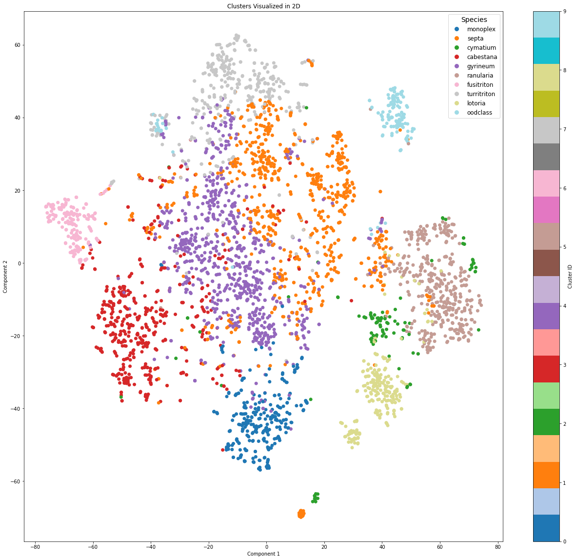
Figure 4: Scatterplot represents clusters formed by the CNN extracted fatures, using tSNE for dimension reduction.
The dispersion of OOD samples reflects the model's ability to treat them as different from the ID classes, which is desirable in tasks
such as OOD detection. The results of Lehmann and Ebner, M [17] corroborate these findings.
The distinct boundaries of the ID clusters further support this by making it easier to flag samples falling outside
the ID clusters as OOD. However, the spread of OOD samples also highlights the inherent challenge of dealing with highly heterogeneous data,
where some samples may occasionally approach the boundaries of ID clusters.
This analysis demonstrates that the feature extractor distinguishes between ID and OOD samples. The insights gained from this clustering
behavior make it clear that the approach to include an OOD class in the training is a valid approach.
Confidence-Based Method: Providing the user hints about the confidence of the categorization
As a first step in OOD detection, we provide the user with feedback on the classification results. While softmax probabilities offer valuable insights to AI experts, they may not be intuitive for users of a CNN model. To address this, we classify the probabilities into four confidence categories, making it easier for users to interpret the model's outputs:- High confidence: The model is highly confident in its classification result.
- Probable: The model is reasonably confident that the classification is correct.
- Possible: The model has average confidence in the classification result.
- Rejected: The model indicates that no reliable identification is possible.
Maximum percentage of misclassification accepted for each category
| Category | Max. % misclassification | Example of a possible range of probabilities (depends on the model) |
|---|---|---|
| "High confidence | < 1% | 1.0-0.9 |
| Probable | 1 - 5 % | 0.9 - 0.7 |
| Possible | 5 - 10 % | 0.7 - 0.5 |
| Rejected | > 10 % | < 0.5 |
- Correctly Classified: Samples where the ground truth matches the predicted category, and the probability is higher than FP.
- Misclassified: Samples where the ground truth differs from the predicted category, but the predicted probability is higher than FP.
- Unknown Class: Samples with probabilities lower than FP are assigned to the unknown category.
Discussion
This article examined the possibility to detect Out-Of-Distribution (OOD) images in the hierarchical CNN for Identifyshell.org From the many methods available to detect OOD images, 2 methods are retained and examined in this article. Our initial goal is to identify OOD images, the next steps will be more advanced methods for Outlier Detection and Novel Class Discovery (NCD) [14].
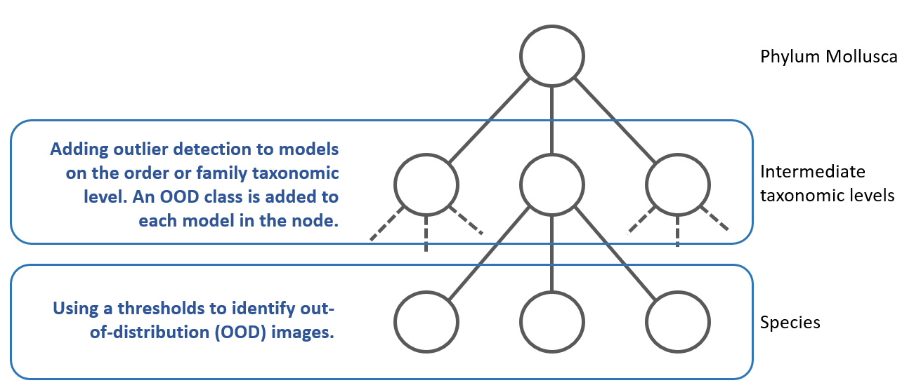
Figure 4: Including OOD detection in the hierarchy of CNNs.
Developing individual state-of-the-art methods for OOD detection is valuable, but each method often comes with its own set of strengths and weaknesses. As a result, combining several methods can often yield superior results compared to relying on any single approach. This is because the strengths of one method can compensate for the weaknesses of another. Numerous examples in machine learning literature demonstrate that method combinations frequently outperform individual techniques [15]. In this paper we have combined 2 methods; outlier detection and thresholds.
OOD and the hierarchy
One significant challenge of hierarchical models is the occurrence of error propagation, a phenomenon where an incorrect decision or
misclassification at an earlier stage of the hierarchy negatively impacts subsequent stages. This cascading effect can substantially
compromise the overall performance of the model. In taxonomic classification tasks, for instance, a misstep at the phylum or order level
can lead to an input being routed down the wrong branch of the hierarchy. As a result, subsequent classifications at the family, genus,
or species levels are based on a flawed foundation, making recovery from the initial error impossible. For example, an image misclassified
at the order level may end up being processed by the wrong family or genus model, leading to an entirely incorrect species identification.
Incorporating out-of-distribution (OOD) detection into hierarchical models provides a robust solution to this issue. By recognizing inputs
that fall outside the expected categories or distributions at each stage, the system can halt the classification process before significant
errors propagate. Instead of forcing a potentially incorrect classification at lower levels, the model can provide reliable information
at a higher taxonomic level. For instance, the process may stop after correctly identifying the order or family, acknowledging the
system's limitations rather than proceeding to make erroneous genus or species-level predictions.
This approach enhances the overall reliability and transparency of the model. It prevents the system from confidently producing incorrect
results and instead ensures that only accurate and well-supported classifications are delivered. Moreover, OOD detection allows for the
special handling of ambiguous or unexpected inputs, which may be flagged for further review or directed to alternative systems designed to
deal with edge cases. By mitigating the risk of cascading errors, hierarchical models equipped with OOD detection become more robust and
better suited to handle complex classification tasks.
As previously mentioned, one of the significant advantages of using hierarchical CNNs is the relative ease of collecting
Out-of-Distribution (OOD) images. In a hierarchical taxonomy, the in-distribution of one taxonomic node inherently serves as
the OOD data for other nodes in the hierarchy. This natural overlap simplifies the process of obtaining OOD datasets, as the model
can leverage already-available images from adjacent or parent taxonomic groups without requiring additional data collection efforts.
In contrast, traditional OOD detection methods often face the challenge of acquiring high-quality, diverse OOD datasets.
This process is typically labor-intensive, requiring careful curation to ensure that the outliers represent realistic
scenarios the model might encounter in deployment. Such datasets must avoid biases that could compromise the model's
generalizability, adding further complexity to the task. However, these challenges do not apply to our hierarchical CNN
framework, as the hierarchical structure inherently provides a built-in mechanism for generating OOD data.
Conclusions and further work
This study demonstrates that integrating Out-of-Distribution (OOD) detection into hierarchical convolutional neural networks (CNNs) enhances their robustness and reliability in open-world scenarios. By identifying and handling unseen Mollusca species, the system mitigates misclassification errors that arise when encountering novel inputs, ultimately improving the utility of CNN-based shell identification models. The inclusion of OOD detection enables the model to separate in-distribution from out-of-distribution samples, which is crucial for ensuring accurate classification while providing meaningful feedback to end-users.While the study establishes a baseline, future work could focus on refining these techniques by employing advanced novelty detection methods, such as energy based thresholds, distance metrics, contrastive learning or self-supervised tasks, to further improve OOD detection accuracy. Note that the goal was to reject unseen classes, but the next step should be to detect novel classes (new species). This ongoing development would pave the way for more reliable and scalable AI systems in biodiversity research and beyond.
References
- [1] Shu, Lei et al. Unseen Class Discovery in Open-world Classification 10.48550/arXiv.1801.05609, (2018)
- [2] Abhijit Bendale and Terrance Boult. Towards open world recognition Proceedings of the IEEE Conference on Computer Vision and Pattern Recognition, pp. 1893–1902, (2015)
- [3] Jingkang Yang et al. Generalized Out-of-Distribution Detection: A Survey International Journal of Computer Vision. 132. 5635-5662. 10.1007/s11263-024-02117-4, (2024)
- [4] S. Ben-David et al. A theory of learning from different domains Machine Learning 79(1-2):151-175, (2010)
- [5] N. Penpong et al. Attacking the out-of-domain problem of a parasite egg detection in-the-wild Heliyon 10(4):e26153. doi: 10.1016/j.heliyon.2024.e26153, (2024)
- [6] A. Krizhevsky, I. Sutskever, and G. E. Hinton Imagenet classification with deep convolutional neural networks NIPS, (2012)
- [7] C. C. Aggarwal and P. S. Yu Outlier detection for high dimensional data ACM SIGMOD Record. 30. 10.1145/376284.375668, (2001)
- [8] L. Ruff et al. A unifying review of deep and shallow anomaly detection Proceedings of the IEEE 109(5), 756-795, (2021)
- [9] M. A. Pimentel et al. A review of novelty detection Signal Processing 99,215-249, (2014)
- [10] T. E. Boult et al. Learning and the unknown: Surveying steps toward open world recognition AAAI 33(1), (2019)
- [11] Dan Hendrycks and Kevin Gimpel A Baseline for Detecting Misclassified and Out-ofDistribution Examples in Neural Networks ICLR, (2017)
- [12] Guo, C. et al. On Calibration of Modern Neural Networks Proceedings of the 34th International Conference on Machine Learning (ICML), (2017)
- [13] Nguyen, A. et al. Deep Neural Networks are Easily Fooled: High Confidence Predictions for Unrecognizable Images. Proceedings of the IEEE Conference on Computer Vision and Pattern Recognition (CVPR), (2015)
- [14] Troisemaine, C. et al Novel Class Discovery: an Introduction and Key Concepts 10.48550/arXiv.2302.12028, (2023)
- [15] Mohandes, M. et al Classifiers combination techniques: A comprehensive review IEEE Access, 6:19626–19639, (2018)
- [16] Vernekar, S. et al. Analysis of Confident-Classifiers for Out-of-distribution Detection 10.48550/arXiv.1904.12220, (2019)
- [17] Lehmann, D. & Ebner, M. Layer-Wise Activation Cluster Analysis of CNNs to Detect Out-of-Distribution Samples ICANN2021, 175, v2, (2021)
- [18] Kingma, D. P., & Welling, M. Auto-Encoding Variational Bayes jInternational Conference on Learning Representations (ICLR)., (2014)
- [19] Ren, J. et al. Likelihood Ratios for Out-of-Distribution Detection. Advances in Neural Information Processing Systems (NeurIPS)., (2019)
- [20] Lee, K., et al. A Simple Unified Framework for Detecting Out-of-Distribution Samples and Adversarial Attacks Advances in Neural Information Processing Systems (NeurIPS)., (2018)
- [21] Liu, W., et al. Energy-Based Out-of-Distribution Detection Advances in Neural Information Processing Systems (NeurIPS). (2020)
- [21] Fort, S., et al. Deep Ensembles: A Loss Landscape Perspective arXiv preprint., (2020)
- [22] Golan, I., & El-Yaniv, R. Deep Anomaly Detection Using Geometric Transformations. Advances in Neural Information Processing Systems (NeurIPS)., (2018)
- [23] Liang, S., et al. Enhancing The Reliability of Out-of-Distribution Image Detection in Neural Networks. International Conference on Learning Representations (ICLR)., (2018)