Analyzing Intra- and Inter-Class Variability and Detecting Outliers in CNN Seashell Image Classification Models
Published on: 14 March 2025
Abstract
Accurate species identification from images is critical for biodiversity monitoring and ecological research. We developed a convolutional neural network (CNN) model to classify Mollusca images from the genus Bufonaria, a taxonomic group characterized by intra-species variability and inter-species similarity. Using a curated dataset of 1,723 images spanning nine Bufonaria species, we trained and evaluated a CNN based on the EfficientNetV2B2 architecture. The model achieved a validation accuracy of 94.8% and F1 scores above 0.95 for most species, demonstrating its effectiveness in capturing subtle morphological distinctions. We analyzed the learned feature space using cosine similarity on high-dimensional embeddings extracted from the penultimate layer of the network. This allowed us to quantify intra-class variability, investigate the influence of image viewpoint, and assess inter-class separability. Outlier detection using k-nearest neighbor analysis revealed that certain images deviated strongly from their class distribution — often due to mislabeling, poor image quality, or atypical shell morphology. Surprisingly, removing these outliers did not consistently improve performance; in some cases, it degraded it, highlighting the nuanced role that atypical examples play in CNN training. Furthermore, we explored the implications of feature space structure for open set recognition and few-shot learning, where clear inter-class boundaries and representative embeddings are critical. Our findings suggest that CNNs not only learn to classify species with high accuracy but also capture meaningful structure in feature space that can inform broader applications in ecological image analysis and biodiversity informatics.
Introduction
Automated species identification plays an increasingly critical role in biodiversity monitoring, taxonomy, and ecological research. In marine environments, where manual identification can be time-consuming and expertise-dependent, machine learning offers a scalable and objective alternative. Among marine organisms, mollusks of the genus Bufonaria [1] present a useful case: these gastropods exhibit striking intra-species variability in morphology, coloration, and surface texture, making them both biologically intriguing and challenging to classify accurately from images. Variability introduced by environmental conditions, developmental stages, and photographic viewpoints further complicates the task, even for experienced taxonomists.
Convolutional neural networks (CNNs) have become the state-of-the-art approach for image-based classification, including biological and taxonomic datasets. CNNs are capable of learning high-dimensional feature representations that capture complex visual patterns far beyond what traditional descriptors offer. However, their success relies heavily on the quality and structure of the training data. One common challenge arises from intra-class variability, where images of the same species differ due to lighting, orientation, wear, or background clutter. Another stems from inter-class similarity, where closely related species share overlapping morphological features that may lead to confusion. These issues are compounded when mislabeled or noisy data are present — a frequent occurrence in large, semi-curated biological datasets. Surprisingly, recent work and our own findings suggest that naïvely removing outliers or mislabeled samples from the training set does not always lead to improved model accuracy. In fact, such removals can degrade performance, particularly when informative but atypical examples are excluded [12].
In this study, we develop and analyze a CNN-based classification model tailored to the mollusk genus Bufonaria. We systematically investigate how intra- and inter-class variability manifest in the model’s learned feature space, using cosine similarity between high-dimensional feature vectors extracted from the penultimate layer of the network [4]. We further explore the utility of these embeddings for detecting atypical or mislabeled images through k-nearest neighbor–based outlier scoring, and assess the downstream effects of removing such outliers on classification performance. Counterintuitively, we find that aggressive outlier removal — even when some removed images are clearly mislabeled or non-representative — can reduce model accuracy, suggesting that certain forms of variability play a regularizing or generalizing role in CNN training.
Beyond conventional classification, we consider the implications of feature space structure for open set recognition (OSR) [15] and few-shot learning [16] — two scenarios highly relevant to ecological applications where rare or unknown species may be encountered. In OSR, the model must distinguish whether an input belongs to any known class or represents a novel species, a task that benefits from high inter-class separability. Few-shot learning, in contrast, requires models to generalize from only a few examples of a new class; here, the ability to construct meaningful, well-separated class prototypes from sparse data is crucial. Our findings suggest that a detailed understanding of the model’s feature space — including the role of outliers and inter-class geometry — is essential not only for improving classification accuracy, but also for enabling generalization to unseen categories in real-world ecological settings.
Methods
Data Acquisition
Shell images were collected from many online resources, from specialized websites on shell collecting to institutes and universities. One of the largest collections of shell images is available on GBIF. Also online marketplace such as ebay contain a large collection of images. Other large shell image collections are available at , Malacopics, Femorale and Thelsica. A shell dataset created for AI is available [17].
Some online resources have facilities to download images, but most websites require a specialized webscraper. Scrapy , an open source and collaborative framework for extracting the data from websites, is used to create a custom webscraper to extract images and their scientific names. All data was stored in a MySQL database before further processing was performed.
The dataset for the Bufonaria CNN model comprises 1723 shell images representing 9 Bufonaria species (see table II). There are 12 species in the genus Bufonaria (WoRMS or MolluscaBase), but not enough images were found for three species. Species with less than 25 images were removed (see Minimum number of images needed for each species).
Image Pre-processing
All names were checked against WoRMS or MolluscaBase for their validity. Names that were not found in WoRMS/MolluscaBase were excluded for further processing. While a large part of this data quality step was automated, a manual verification (time-consuming) step was also included. In addition to text-based quality control, both automated and manual preprocessing steps were applied to the images. Shells were detected in all images and cut out of the original image, having only 1 shell on each image. Other objects on the raw images (labels, measures, hands holding a shell, etc.) were removed. When appropiate the background was changed to a uniform black background. A square image was made by padding the black background. All shells were resized (400 x 400 px).
Model Training
For this study, Python (version 3.10.12) was used. The EffiecientNetV2B2 pre-trained models were used. (see Identifying Shells using Convolutional Neural Networks: Data Collection and Model Selection) Table 2 lists the hyperparameters. The models were trained using a batch size of 64 samples, and the number of epochs used was 50. The learning process was initiated with an initial learning rate of 0.0005 and the Adam optimiser was utilised for efficient weight updates. Two callbacks were used, one to monitor the validation loss and decreasing the learning rate , a second callback for early stopping. Both callbacks were applied to prevent the model from over-fitting. Fine-tuning the model was performed as described before. The top 30 layers of the model were unfrozen.
Table II. Hyperparameters
| Hyperparameter | Value | Comments |
|---|---|---|
| Batch Size | 64 | |
| Epochs | 50 | The number of epochs determines how many times the entire training dataset is passed through the model. Because early-stopping is used, often less than 50 epochs were needed. |
| Optimizer | Adam | The optimizer determines the algorithm used to update model weights during training. |
| Learning Rate | 0.0005 |
The validation loss was monitored and adjusted reduce_lr = keras.callbacks.ReduceLROnPlateau(monitor='val_loss', factor=0.1, patience=3, min_lr=1e-6) |
| Loss | Categorical Cross-entropy | |
| Regularization | 0.001 |
Evaluation Metrics
The evaluation of the performance of the CNN models was carried out by using standard metrics for classification: accuracy, precision, recall, and F1 score,
which are defined by [7] in terms of the number of FP (false positives); TP (true positives); TN (true negatives); and FN (false negatives) as follows:
Precision = TP/(TP + FP)
Recall = TP/(TP + FN)
F1-Score = 2 × (Precision × Recall)/(Precision + Recall)
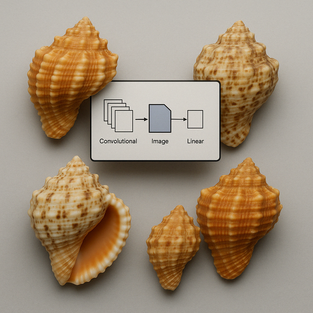
Feature vectors from the the penultimate layer of the trained Bufonaria CNN model
To analyze the internal representations learned by the Bufonaria CNN model, we extracted high-dimensional feature vectors from the penultimate layer of the trained network.
These embeddings capture rich semantic information about each image while abstracting away from pixel-level details. The model was implemented and trained using TensorFlow,
and feature vectors were obtained using Keras’ Model subclassing, where a truncated version of the network outputs activations from the final convolutional or dense layer
prior to classification. Each image in the dataset was passed through the network in inference mode, and the resulting feature vector (1408 dimensions) was stored for
further analysis.
To quantify similarity between images, we computed pairwise cosine similarity between feature vectors.
For each image , compute similarity to all other images in the same class:
and are the feature vectors (or embeddings) corresponding to image and image , respectively. These are extracted from the penultimate layer of the trained CNN and represent the model's internal encoding of visual characteristics in a high-dimensional space.
Cosine similarity measures the cosine of the angle between two vectors in the embedding space, and is particularly well-suited for high-dimensional data where the magnitude of the vectors is less informative than their direction. It was calculated using the sklearn.metrics.pairwise.cosine_similarity function from scikit-learn. Cosine distance (1 - similarity) was used when required for clustering, outlier detection, or visualization purposes. This approach allowed us to evaluate both intra-class cohesion and inter-class separation based on the learned feature representations, providing a model-centric view of image similarity beyond what can be captured by raw pixel comparisons.
Outlier detection
To assess intra-class consistency and detect potential annotation errors or atypical images, we performed outlier analysis on the feature vectors.
For each image, we computed its high-dimensional embedding and grouped the dataset by species (i.e., class label). Within each species, we applied a k-Nearest Neighbors (kNN) approach
using cosine distance to estimate local density in feature space. Specifically, for each image, we calculated the average cosine distance to its five nearest neighbors belonging to
the same species. This intra-class distance served as an outlier score, with higher values indicating images that deviated from the typical structure of their class.
To account for variability across species, we determined outlier thresholds separately for each species by computing the 95th percentile of the intra-class outlier score distribution.
Images exceeding this threshold were flagged as class-specific outliers. We visualized the distribution of scores per species using boxplots and summarized the variability of each
class by computing the standard deviation and maximum outlier score. This approach allowed us to identify species with unusually broad internal variability as well as individual
images that may represent mislabelled examples, poor-quality data, or biologically atypical instances.
All analyses were implemented in Python using standard scientific computing libraries including NumPy, pandas, scikit-learn (for kNN and distance calculations), and
seaborn/matplotlib for visualization.
Results
The Bufonaria model
The dataset for the Bufonaria CNN model comprises 1723 shell images representing 9 Bufonaria species (see table II). There are 12 species in the genus Bufonaria (WoRMS or MolluscaBase), but not enough images were found for two species. Species with less than 25 images were removed (see Minimum number of images needed for each species). A third species (B. subgranosa) was removed from the final model because this species was confused with Bufonaria rana (data not shown). B. subgranosa was previously considered to be a synonym of B. rana (see wikipedia - accessed 4-Apr-2025). Note also the removal of the species B. margaritula, accepted as Bursina margaritula (Deshayes, 1833) The Bufonaria CNN model shows a good performance with a 95% validation accuracy, indicating its excellent ability to generalize to unseen data. A summary of the results of the overall model is given in table I.
Table I. Training Results
| Metrics | Value | Comments |
|---|---|---|
| Validation accuracy | 0.948 | |
| Validation loss | 0.206 | |
| Training accuracy | 0.979 | |
| Training loss | 0.108 | |
| Weighted Average Recall | 0.956 | |
| Weighted Average Precision | 0.956 | |
| Weighted Average F1 | 0.956 |
The validation loss of 0.206 confirms effective generalization without significant overfitting. Additionally, the training accuracy reached 97.9%, and the training loss was 0.108, both of which reflect efficient learning and optimization during the training process. Furthermore, the model showed balanced predictive capabilities across precision, recall, and the F1 score, each yielding 95.6%, highlighting the overall robustness and reliability of the classification performance. These results collectively confirm that the Bufonaria CNN model effectively captures distinguishing features necessary for accurate predictions. Metrics for each species are shown in table II.
Table II. Metrics for each species
| Species | # images | Recall | Precision | F1 |
|---|---|---|---|---|
| Bufonaria cavitensis (Reeve, 1844) | 179 | 0.893 | 0.926 | 0.909 |
| Bufonaria cristinae Parth, 1989 | 71 | 0.786 | 0.846 | 0.815 |
| Bufonaria crumena (Lamarck, 1816) | 278 | 0.964 | 0.964 | 0.964 |
| Bufonaria echinata (Link, 1807) | 102 | 0.958 | 1.000 | 0.979 |
| Bufonaria elegans (G. B. Sowerby II, 1836) | 75 | 1.000 | 0.933 | 0.966 |
| Bufonaria foliata (Broderip, 1825) | 170 | 1.000 | 1.000 | 1.000 |
| Bufonaria granosa (K. Martin, 1884) | 262 | 0.979 | 0.922 | 0.949 |
| Bufonaria rana (Linnaeus, 1758) | 404 | 0.949 | 0.959 | 0.954 |
| Bufonaria thersites (Redfield, 1846) | 182 | 1.000 | 1.000 | 1.000 |
The Bufonaria CNN model showed strong and consistent classification performance across most species, with metrics varying slightly depending on species and training sample sizes.
The model achieved perfect or near-perfect results for species with distinct visual features, such as Bufonaria thersites and Bufonaria foliata,
with 100% recall, precision, and F1, and Bufonaria echinata,
with consistent metrics above 95.8%. High accuracy was also noted in species with larger datasets like Bufonaria rana (recall: 94.9%, precision: 95.9%, F1: 95.4%) and
Bufonaria crumena (recall/precision/F1: 96.4%), reflecting reliable predictive ability likely supported by abundant training examples.
Some species with fewer training examples exhibited more variability. For instance, Bufonaria cristinae (recall: 78.6%, precision: 84.6%, F1: 81.5%),
showed lower results, likely due to the limited number of images.
Confusion matrix
The confusion matrix, shown in figure 1, confirms the strong overall performance of the Bufonaria CNN model, while highlighting specific areas of confusion among certain species. The matrix clearly illustrates high accuracy along the diagonal, indicating correct classifications, consistent with previously reported precision, recall, and F1 scores.
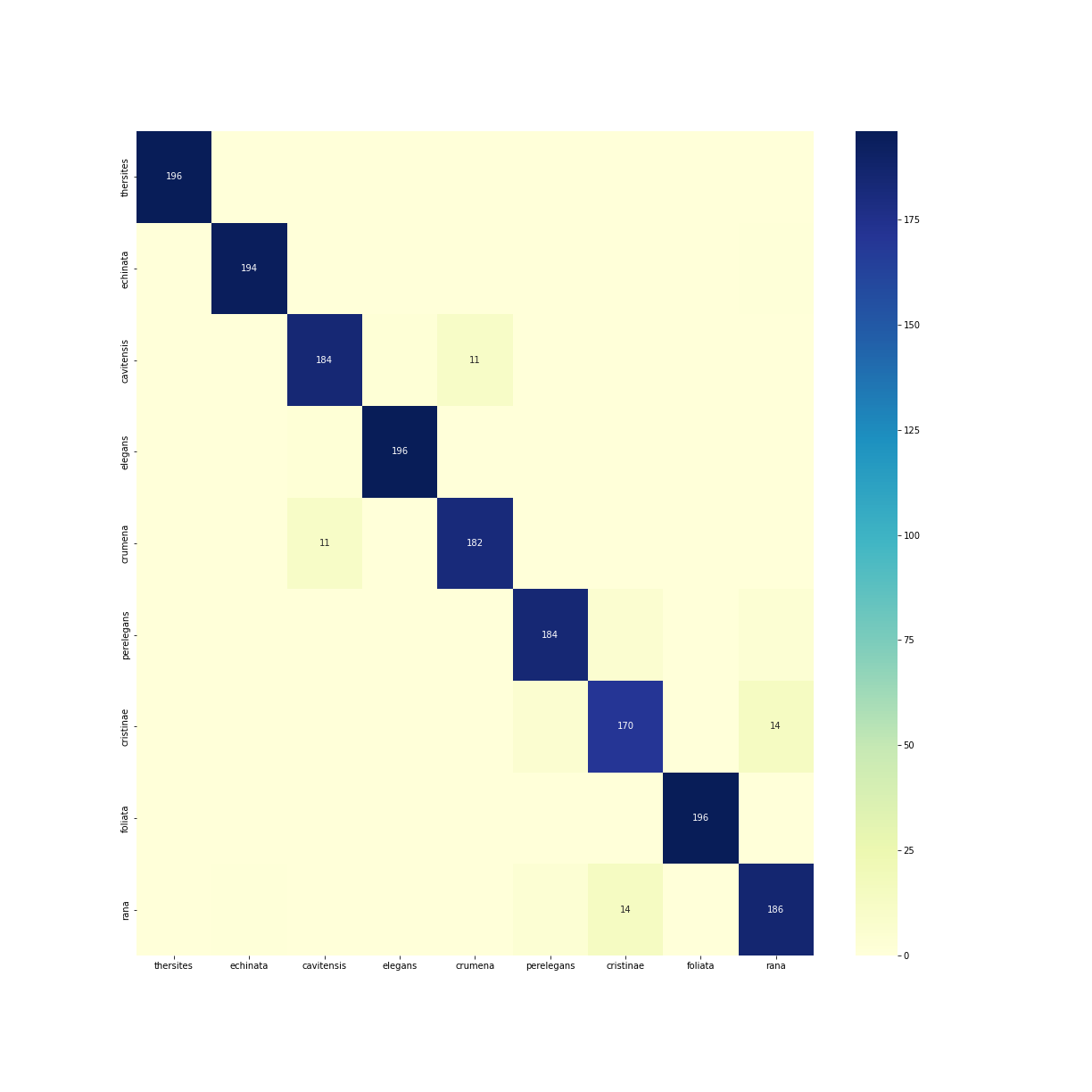
Figure 1: Confusion matrix
However, some notable confusions are present. A small number of images from Bufonaria cristinae and Bufonaria rana, are incorrectly classified, confirming the previously described lower recall/precision for Bufonaria cristinae.
Overall, the confusion matrix supports earlier findings, highlighting strong accuracy across most classes while clarifying specific areas of minor confusion, typically among visually similar species or species with fewer training examples.
Intra-class variability and viewpoints
We extracted feature vectors from the penultimate layer of our model and computed the pairwise cosine similarity between all images within each class. To visualize these similarities, we applied t-SNE [2], a dimensionality reduction technique well-suited for exploring high-dimensional data. This allowed us to project the feature vectors into a two-dimensional space, making it easier to observe the relative positioning of images within a given class or species based on their similarity.To further interpret the visualizations, we annotated each image with its corresponding viewpoint [3] and color-coded the scatter plot accordingly. This helps reveal whether images with similar viewpoints tend to cluster together in feature space. An example of this visualization is shown in Figure 2, which displays the t-SNE projection for Bufonaria elegans and Bufonaria cavitensis.
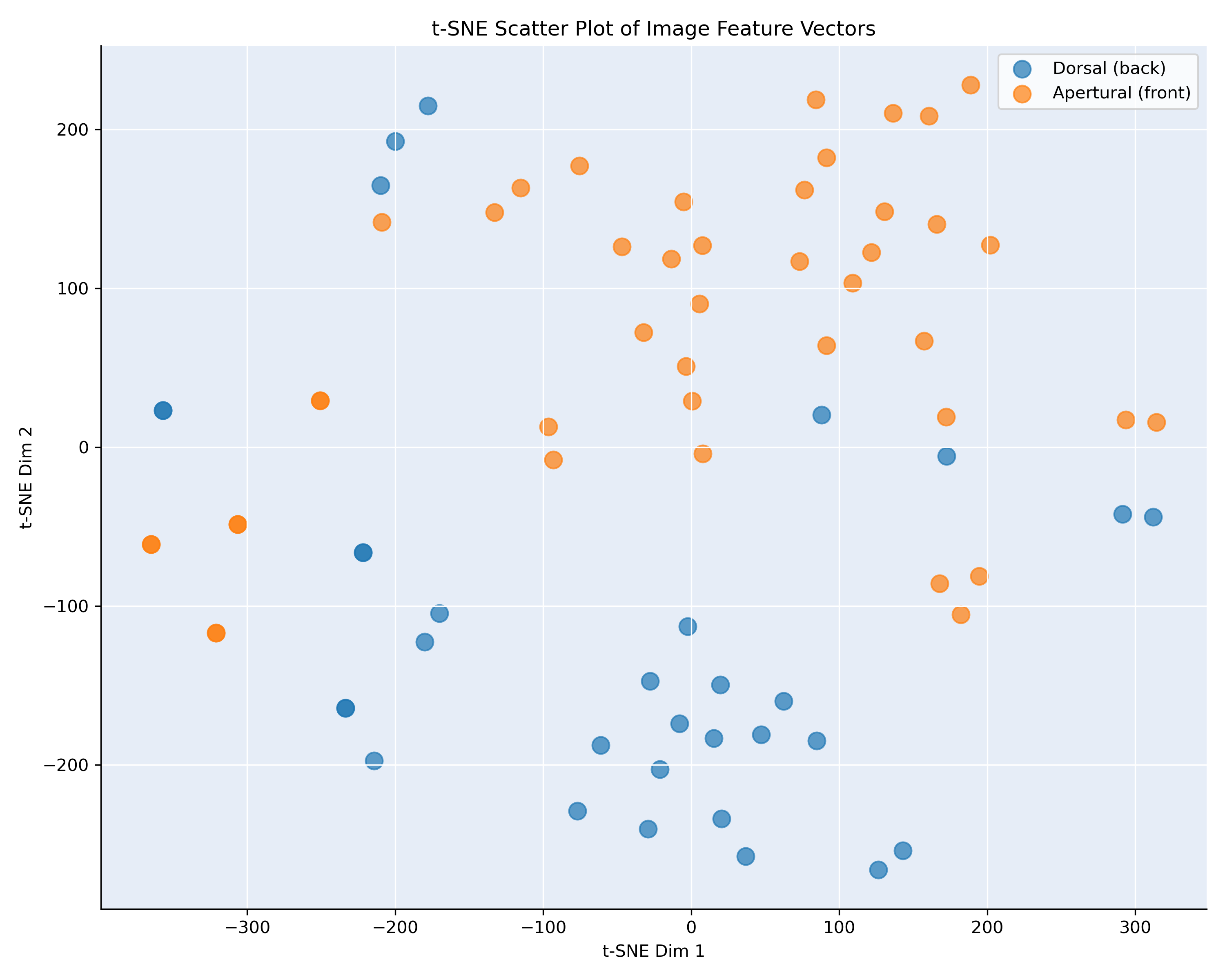
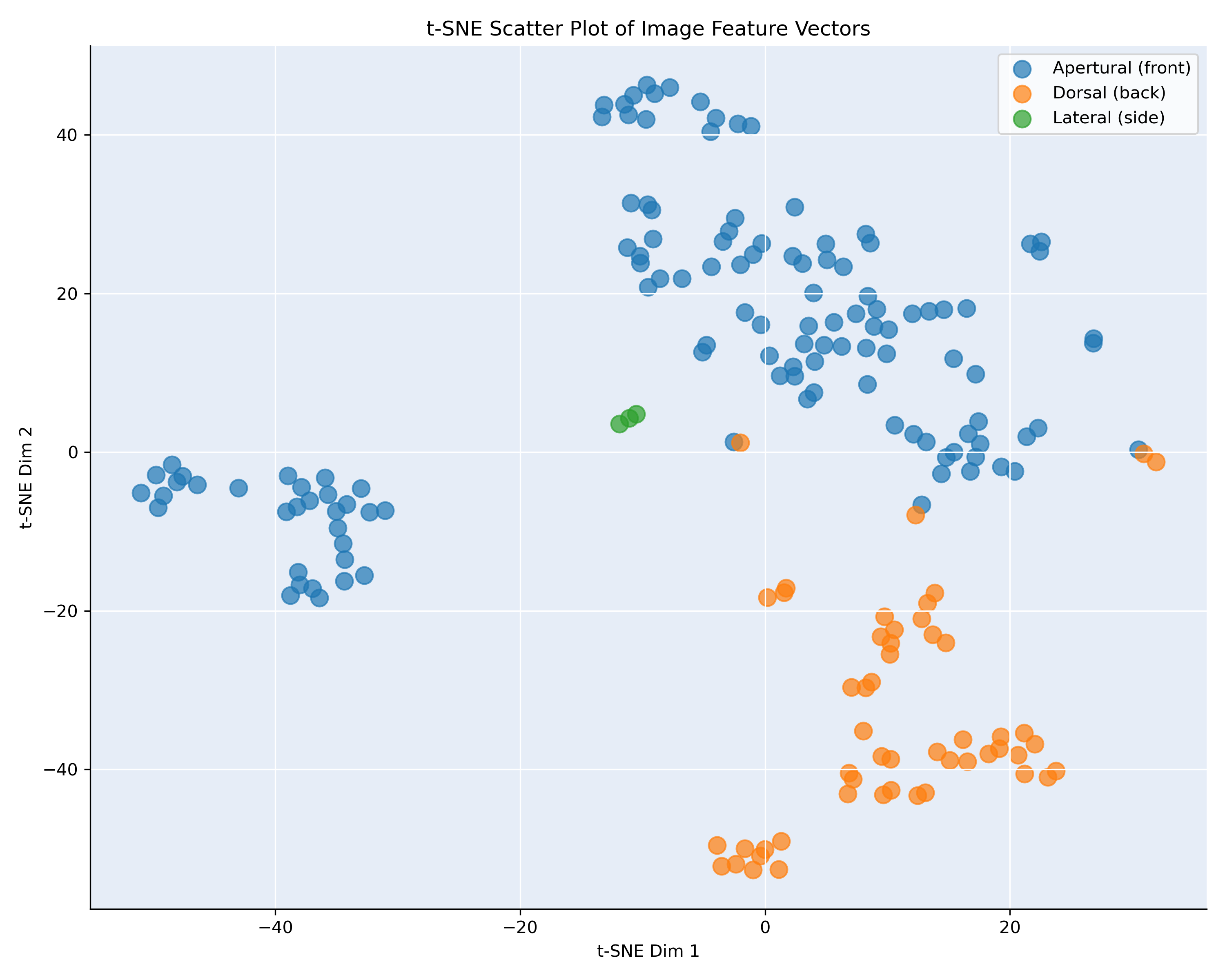
Figure 2: t-SNE visualization, showing the similarity of the images of B. elegans and cavitensis
Figure 2 presents a t-SNE projection of image feature vectors for the species Bufonaria elegans (75 images) and Bufonaria cavitensis (179 images),
based on pairwise cosine similarity computed from
the penultimate layer of the neural network. Each point corresponds to a single image, and colors indicate the annotated viewpoint: apertural (front) in orange and
dorsal (back) in blue.
The distribution reveals a clear separation between the two viewpoints. Most images cluster according to their orientation, with dorsal and apertural views forming
distinct regions in the embedded space. This indicates that the model’s high-level feature representation is strongly influenced by the viewpoint of the specimen.
The grouping suggests that images taken from similar angles result in more similar feature vectors, even within a single species.
Such separation confirms that the viewpoint contributes significantly to the learned visual similarity and should be accounted for in downstream tasks such as
clustering, classification, or species comparison. Moreover, it highlights the importance of viewpoint normalization or augmentation in datasets where intra-class
variance is driven by imaging perspective rather than morphological differences.
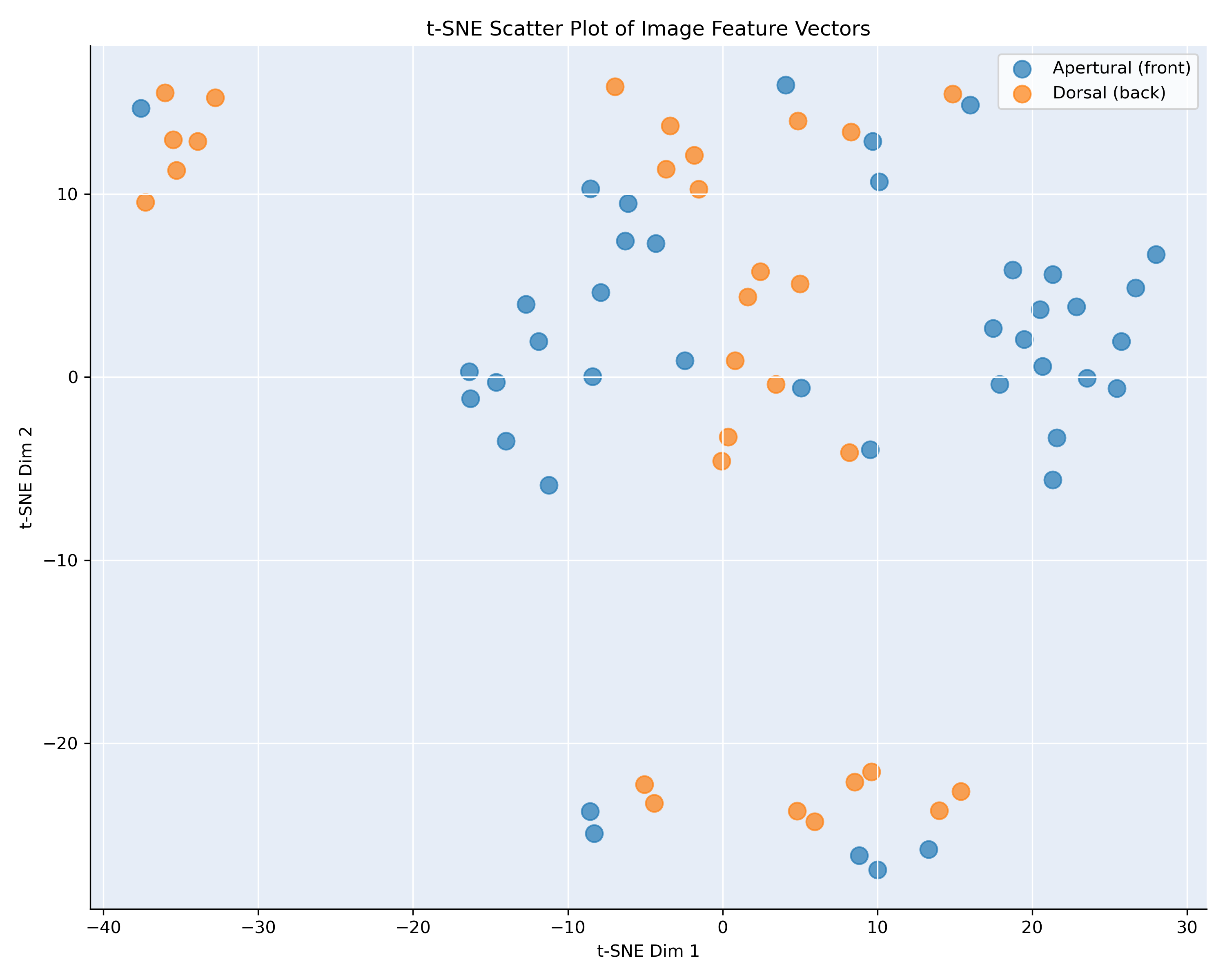
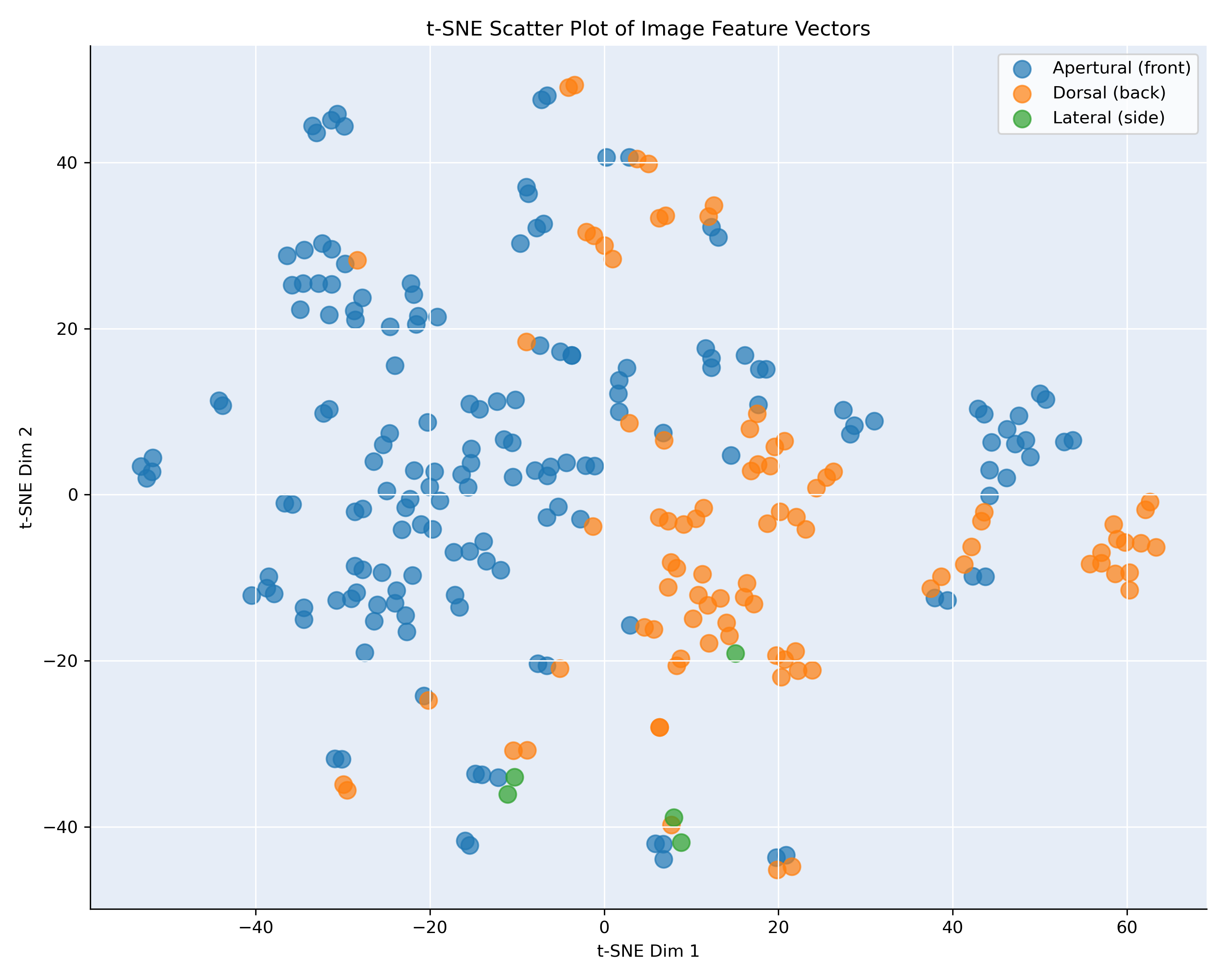
Figure 3: t-SNE visualization, showing the similarity of the images of B. cristinae and granosa
Figure 3 shows the t-SNE projection of the feature vectors for Bufonaria cristinae (71 images) and Bufonaria granosa (262 images), computed from the penultimate layer of the neural network
and color-coded by image viewpoint: apertural (front) in blue and dorsal (back) in orange.
In contrast to B. elegans and B. cavitensis (Figure 2), the embeddings for B. cristinae and B. granosa display a less pronounced separation between viewpoints.
While some clusters appear to be viewpoint-specific there is substantial overlap between apertural and dorsal images in other regions. This suggests that, for these
two species, the network’s learned features are less strongly influenced by viewpoint.
The mixed clusters may indicate that certain features extracted from different viewpoints are still highly similar, possibly due to repetitive patterns or
structural symmetry in the shell. Alternatively, it may reflect greater variation within a viewpoint, reducing the network’s ability to group them distinctly.
These results highlight species-level differences in how viewpoint affects the learned representation. They also underscore the need for careful consideration
of viewpoint during training, especially for species with subtle morphological differences across views.
The variability is calculated for all species and given in Table
CNN models per viewpoint
The findings presented above prompted the development of separate CNN models tailored to each viewpoint. Table III presents a comparison of the classification accuracy achieved by these viewpoint-specific models versus a single model trained on the combined set of all viewpoints.Table III. Metrics for each species
| model with all viewpoints | model with only apertural view | model with only dorsal view | ||||
|---|---|---|---|---|---|---|
| Species | # images | F1 | # images | F1 | # images | F1 |
| Bufonaria cavitensis (Reeve, 1844) | 179 | 0.909 | 124 | 0.957 | 52 | 0.960 |
| Bufonaria cristinae Parth, 1989 | 71 | 0.815 | 41 | 0.750 | 30 | 0.909 |
| Bufonaria crumena (Lamarck, 1816) | 278 | 0.964 | 139 | 0.824 | 127 | 0.870 |
| Bufonaria echinata (Link, 1807) | 102 | 0.979 | 51 | 0.952 | 44 | 0.824 |
| Bufonaria elegans (G. B. Sowerby II, 1836) | 75 | 0.966 | 43 | 1.000 | 32 | 1.000 |
| Bufonaria foliata (Broderip, 1825) | 170 | 1.000 | 81 | 1.000 | 69 | 1.000 |
| Bufonaria granosa (K. Martin, 1884) | 262 | 0.949 | 166 | 0.903 | 90 | 0.757 |
| Bufonaria rana (Linnaeus, 1758) | 404 | 0.954 | 254 | 0.887 | 130 | 0.792 |
| Bufonaria thersites (Redfield, 1846) | 182 | 1.000 | 125 | 1.000 | 53 | 0.960 |
| Overall | 1723 | 0.956 | 1024 | 0.907 | 627 | 0.856 |
Table III presents the F1 scores obtained for each Bufonaria species using three different CNN model configurations: a model trained on images from all viewpoints,
and two separate models trained exclusively on apertural or dorsal views. The results reveal clear species-specific trends in how viewpoint affects classification
performance.
For several species — including Bufonaria elegans and Bufonaria foliata — the viewpoint-specific models achieve perfect or near-perfect F1 scores, matching or exceeding
the performance of the model trained on all viewpoints. Notably, B. elegans achieves an F1 score of 1.000 for both the apertural-only and dorsal-only models,
compared to 0.966 when using all viewpoints. This aligns with the t-SNE visualization in Figure 1, where a strong separation between viewpoints is observed,
suggesting that training a unified model across both orientations may introduce unnecessary variance into the feature space.
Similarly, Bufonaria cristinae — shown in Figure 2 — demonstrates an inverse trend. The dorsal-only model outperforms both the all-view model and the apertural-only
model (F1 = 0.909 vs. 0.815 and 0.750, respectively). The intermingling of viewpoints in Figure 2 indicates that images from different perspectives may not
be easily distinguishable in feature space, and training a model on a mixed-view dataset could dilute viewpoint-specific discriminative features.
Across the dataset, dorsal-only models often perform comparably to or better than the all-view models, particularly when sufficient training data is
available (e.g., B. cavitensis and B. cristinae). These results support the hypothesis that viewpoint-specific modeling can improve classification
accuracy by reducing intra-class variability and enabling the network to focus on consistent visual cues.
While viewpoint-specific models often yield higher classification performance, as seen for several species in Table III, this improvement must be considered in
light of the associated reduction in training sample size. Dividing the dataset by viewpoint necessarily decreases the number of training examples available
for each model, which can adversely affect generalization — particularly for species with limited representation. For instance, Bufonaria cristinae shows
improved performance when using only dorsal views (F1 = 0.909), but the corresponding apertural - only model performs worse (F1 = 0.750), likely due to the
smaller number of samples (41 images). Conversely, species with larger and more balanced datasets, such as B. cavitensis and B. elegans, benefit from
viewpoint-specific training without significant performance loss, achieving high F1 scores across all configurations.
This highlights a key trade-off: while training separate models per viewpoint can reduce intra-class variability and improve discriminative power,
it may also lead to data sparsity, especially for rare species or underrepresented views. Therefore, the decision to adopt viewpoint-specific models
should be guided not only by observed viewpoint separability (as suggested by the t-SNE plots), but also by the availability of sufficient training data to
support robust model learning.
Inter-class variability
We analyzed inter-class similarity in the same way get more information on the similarity of the classes in feature space. We computed the pairwise cosine similarity between all images. Again, we applied t-SNE [2], to explore the feature vectors into a two-dimensional space, making it easier to observe the relative positioning of images within a given class or species based on their similarity. The t-SNE vizualisation is given in figure 4.
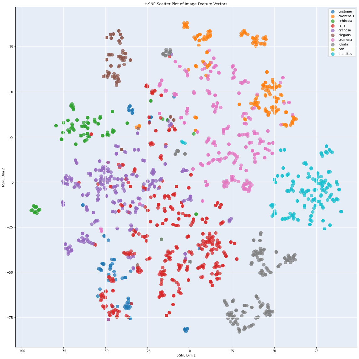
Figure 4: t-SNE visualization, showing the interclass similarity for Bufonaria
This scatter plot in figure 4 shows the t-SNE projection. Each point corresponds to an individual image, and points are color-coded by species label. The spatial arrangement of points reflects the learned similarity in the CNN feature space: images of the same species form localized clusters, while species with distinct visual characteristics are well separated. Notably, several species (e.g., cristinae, granosa, cavitnessis, and thersites) form tight, well-separated clusters, indicating high intra-class compactness and strong inter-class separation. Conversely, partially overlapping regions (e.g., between B. rana and B. cumanea) suggest that the CNN has learned similar representations for those classes, possibly reflecting shared morphological features or challenging intra-class variability.
The heatmap (figure 5) visualizes the pairwise cosine similarity between species-level feature centroids computed from CNN feature vectors. Each cell reflects the
similarity between the average embedding of two species, with higher values (closer to 1) indicating greater similarity in the model’s learned feature space. Diagonal
values are 1.00 by definition, representing self-similarity.
The matrix reveals varying degrees of inter-species similarity. Notably, some species pairs, such as B. cristinae and B. granosa, as well as B. foliata and B. granosa,
exhibit high cosine similarity (≥ 0.85), suggesting that their feature representations are closely aligned, which could explain potential confusion during classification.
In contrast, species like B. rana and B. thersites display low similarity (< 0.3), indicating that the model has learned distinct feature representations for these classes.
These insights complement traditional confusion matrix analysis by offering a feature-space-level perspective on class separability.
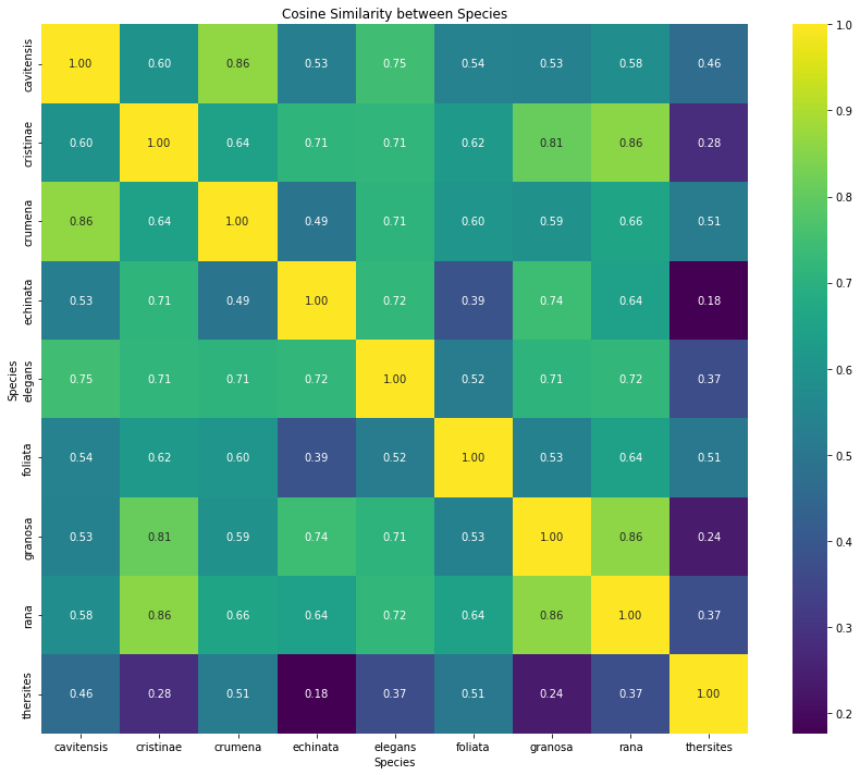
Figure 5: Cosine distance (1 - similarity) between species. Heatmap visualization
The dendrogram (figure 6) presents a hierarchical clustering of species based on cosine distance (1 – similarity) between their class centroids. Species that are closer in the CNN’s feature space are grouped together at lower linkage distances. The tree structure highlights clusters of visually or morphologically similar species. For instance, the close clustering of B. cavitnessis, B. granosa, and B. foliata suggests these classes are tightly related in the model’s internal representation. The hierarchical structure helps identify broader groupings and potential taxonomy-like relationships learned by the CNN, even in the absence of explicit hierarchical labels. This information can guide refinement of class definitions, identify candidates for merging or relabeling, or inform model design in applications such as open-set recognition and few-shot learning.
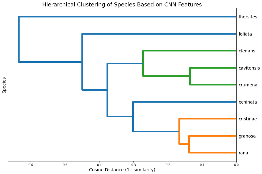
Figure 6: Cosine distance (1 - similarity) between species. Dendogram
Outlier detection
While the viewpoint of a shell in the image significantly influences intra-class variability, several other parameters also contribute to this variability. These include differences in lighting conditions, variations in shell coloration and patterns, varying degrees of wear or damage on the shell surface, background complexity or clutter in the image, and scale variations due to differing distances between the camera and the shell. In addition, misclassification errors themselves significantly contribute to intra-class variability, as incorrectly labeled or ambiguous images can distort feature representations and complicate the accurate identification of consistent patterns within classes.
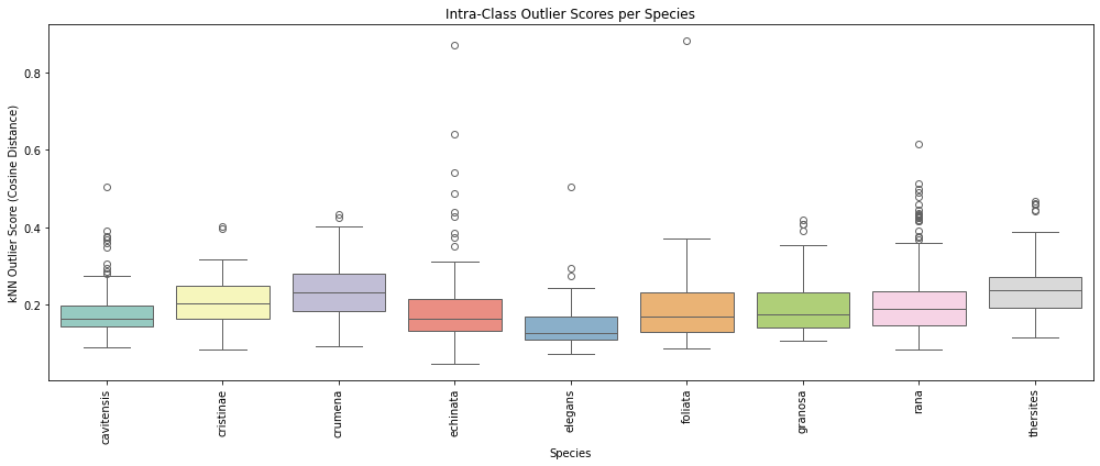
Figure 7: Boxplot showing the outliers by species
Figure 7 presents the distribution of kNN-based outlier scores across all examined species, where each boxplot summarizes the intra-class variability in the learned
CNN feature space. For each species, the boxplot shows the spread of cosine-based outlier scores relative to the species' own internal feature structure. These scores
represent how far individual images deviate from their local neighborhood within the same class.
As seen in the figure, several species exhibit tightly clustered distributions with minimal variability (e.g., B cristinae, B. rana), suggesting consistent feature representations
and relatively homogeneous image sets. In contrast, other species such as B. echinata and B. cavitnessis display broader distributions and a greater number of high-score outliers,
indicative of higher intra-class diversity or the presence of mislabeled or atypical samples. Notably, these species also show a substantial number of outliers beyond the upper
whisker, pointing to individual images that are substantially less similar to their class peers in the feature space.
This pattern highlights the uneven distribution of feature-space variability across classes and reinforces the need for per-species treatment in quality control and error detection.
The boxplot thus provides a concise visual summary of intra-class structure and the reliability of training data across species.
Table IV. Variability metrics per species
| Species | Average kNN outlier score | Std. dev. kNN outlier score | Outlier Percentage |
|---|---|---|---|
| Bufonaria cavitensis (Reeve, 1844) | 0.177 | 0.059 | 5.028 |
| Bufonaria cristinae Parth, 1989 | 0.206 | 0.068 | 5.633 |
| Bufonaria crumena (Lamarck, 1816) | 0.234 | 0.065 | 5.036 |
| Bufonaria echinata (Link, 1807) | 0.194 | 0.123 | 5.882 |
| Bufonaria elegans (G. B. Sowerby II, 1836) | 0.148 | 0.062 | 5.333 |
| Bufonaria foliata (Broderip, 1825) | 0.189 | 0.087 | 5.294 |
| Bufonaria granosa (K. Martin, 1884) | 0.191 | 0.062 | 5.343 |
| Bufonaria rana (Linnaeus, 1758) | 0.202 | 0.081 | 5.198 |
| Bufonaria thersites (Redfield, 1846) | 0.244 | 0.071 | 5.494 |
Table IV presents a summary of intra-class variability metrics calculated for each species in the dataset based on kNN-derived outlier scores. For each species, we report
the average outlier score, its standard deviation, and the proportion of images identified as outliers (defined as those above the 95th percentile within their class).
These metrics quantify the degree of internal heterogeneity observed in the CNN feature space for each species.
Species such as Bufonaria echinata and Bufonaria foliata exhibit relatively high standard deviations (0.123 and 0.087, respectively), indicating broader
intra-class spread and potentially greater morphological diversity or inconsistency in imaging conditions. In contrast, species like Bufonaria elegans and
Bufonaria granosa display lower variability, reflecting more cohesive and consistent feature representations. The outlier percentages for all species are close
to the theoretical 5% threshold used during score thresholding, confirming consistent detection criteria across classes.
Training the CNN model without outliers
Table V summarizes the performance of the CNN model across four experimental runs, each involving a different strategy for outlier removal. In the baseline condition (no outlier removal), the model achieved an overall F1 score of 0.948. Three alternative runs progressively removed more outliers: (1) all samples with a kNN-based outlier score above 0.75, (2) samples with a score above 0.50, and (3) the top three outliers per species, as ranked by their intra-class outlier scores.
Table V. Impact of outlier removal on model performance
| Species | No outlier removal | outlier (>0.75) removed | outlier (>0.50) removed | outlier (top 3) removed | ||||
|---|---|---|---|---|---|---|---|---|
| Species | # images | F1 | # images | F1 | # images | F1 | # images | F1 |
| Bufonaria cavitensis (Reeve, 1844) | 179 | 0.909 | 179 | 0.933 | 178 | 0.915 | 176 | 0.839 |
| Bufonaria cristinae Parth, 1989 | 71 | 0.815 | 71 | 0.875 | 71 | 0.839 | 68 | 0.750 |
| Bufonaria crumena (Lamarck, 1816) | 278 | 0.964 | 278 | 0.953 | 278 | 0.925 | 275 | 0.880 |
| Bufonaria echinata (Link, 1807) | 102 | 0.979 | 101 | 0.978 | 99 | 0.978 | 99 | 0.870 |
| Bufonaria elegans (G. B. Sowerby II, 1836) | 75 | 0.966 | 75 | 1.000 | 74 | 1.000 | 72 | 0.933 |
| Bufonaria foliata (Broderip, 1825) | 170 | 1.000 | 169 | 1.000 | 169 | 0.971 | 167 | 0.986 |
| Bufonaria granosa (K. Martin, 1884) | 262 | 0.949 | 262 | 0.889 | 262 | 0.863 | 259 | 0.863 |
| Bufonaria rana (Linnaeus, 1758) | 404 | 0.954 | 404 | 0.927 | 402 | 0.906 | 401 | 0.885 |
| Bufonaria thersites (Redfield, 1846) | 182 | 1.000 | 182 | 0.984 | 182 | 1.000 | 179 | 1.000 |
| Overall | 1723 | 0.948 | 1721 | 0.947 | 1715 | 0.927 | 1696 | 0.894 |
Contrary to expectations, removing more outliers did not consistently improve model performance. The removal of only the most extreme outliers (threshold > 0.75)
yielded a nearly identical overall F1 score (0.947), suggesting that a small number of unrepresentative or mislabeled images had limited negative influence.
However, more aggressive removal strategies — particularly using a lower threshold (> 0.50) or the top three outliers per species — led to a noticeable decline
in performance, with the overall F1 dropping to 0.927 and 0.894, respectively. These results indicate that while extreme outliers may be safely removed without
penalty, the broader removal of samples deemed “atypical” may degrade model generalization.
At the species level, this trend was evident in several cases. For instance, Bufonaria cavitensis and Bufonaria cristinae initially benefited
from modest outlier removal (F1 increasing from 0.909 to 0.933, and from 0.815 to 0.875, respectively), but their F1 scores dropped substantially when more
images were removed in the “top 3” condition (down to 0.839 and 0.750). Similar patterns were observed for B. crumena, B. echinata, and B. rana. These declines
likely result from the removal of rare but informative training examples — images that may appear as statistical outliers but still represent legitimate, diverse
instances within a class.
These findings highlight an important consideration in outlier handling: removing difficult or rare samples indiscriminately may narrow the training distribution,
leading to overfitting on the more common patterns and reduced robustness at test time. In this case, even outliers that were visually confirmed as mislabeled or
non-shell images did not appear to harm the model significantly when present, but their removal reduced the diversity and volume of training data.
Discussion
Addressing Intra-Class Variability: The Case Against Viewpoint-Specific Models
A central challenge in image classification, particularly for objects like shells, is intra-class variability – the phenomenon where objects within the same category exhibit significant visual differences. This variability stems from factors such as viewpoint changes, illumination, pose, background clutter, and even developmental stages, as seen in classifying different leaf o plant species based on growth stage [5]. For our shell identification application, this inherent variability, especially due to viewpoint, raises a practical question: should we train separate Convolutional Neural Network (CNN) models for each distinct viewpoint?
While viewpoint-specific models can sometimes improve classification accuracy, as suggested by our results in Table III, we argue that this approach is impractical for a user-facing shell identification system. The primary drawbacks are usability and scalability. Requiring users to manually identify and input the viewpoint for every image introduces a significant hurdle, diminishing the user experience and limiting the system's accessibility. Furthermore, the performance benefits of viewpoint-specific models are not guaranteed; they are often contingent on having sufficient and balanced training data for each view per species. In cases of limited or imbalanced data, such models might even underperform compared to a single, comprehensive model.
Our finding that a unified model offers better overall robustness aligns with research exploring how CNNs inherently manage intra-class variations. Studies have shown that CNNs learn to organize different object variations within their feature representations. For instance, Wei et al. [4] demonstrated using visualization techniques that higher layers of CNNs can implicitly cluster images from the same class based on attributes like pose and viewpoint, effectively performing unsupervised discovery of these sub-types (e.g., distinguishing side-view from top-view dragonflies) even without explicit viewpoint labels during training. Other research corroborates this, using methods like clustering feature embeddings [6, 7] or analyzing intra-class variance scores [8] to understand how networks represent these internal class structures. While these analysis techniques (including feature visualization and pattern mining [9]) highlight the complexity of intra-class knowledge within CNNs, they also suggest that a single network can learn to accommodate variations like viewpoint.
Therefore, we conclude that the practical advantages of a single, integrated model capable of handling images from any viewpoint outweigh the potential, but often marginal and conditional, accuracy gains from viewpoint-specific models. The modest reduction in accuracy for some species is an acceptable trade-off for enhanced usability and robustness across the entire dataset. Future work might explore automated viewpoint estimation as a pre-processing step, potentially capturing the benefits of viewpoint-aware modeling without sacrificing user convenience.
Inter-Class Variability: Implications for Open Set and Few-Shot Scenarios
Having established that a unified model can effectively handle intra-class variability like viewpoint, the next critical factor is its ability to distinguish between different shell species – a measure of inter-class variability. Our analysis of the feature space geometry in this regard has significant implications beyond standard closed-set classification, particularly for challenging tasks like Open Set Recognition (OSR) and Few-Shot Learning (FSL).
In OSR, the goal is not only to classify known species but also to identify inputs that belong to none of the known classes. This requires a well-structured feature space where class boundaries are clearly defined and inter-class distances are sufficiently large to allow for reliable rejection of unknown inputs. Our analysis of inter-class variability provides insight into how distinct or overlapping the feature embeddings of different shell species are. In cases where classes are tightly clustered or entangled, the model is more prone to false positives under OSR conditions. Conversely, when species are well-separated in the embedding space, the model is better positioned to detect unfamiliar or novel inputs by measuring their distance from known class centroids.
Similarly, few-shot learning — where the model must generalize to new categories with only a handful of labeled examples — also benefits from high inter-class separability. Embedding-based approaches to few-shot learning, such as prototypical [10] or matching networks, rely heavily on the geometry of the feature space learned during training. A feature space with strong inter-class variability and compact intra-class clusters enables the model to construct meaningful prototypes and make accurate predictions even with limited data. Our inter-class analysis can thus guide the design of few-shot learning strategies, such as selecting which base classes to train on, or refining loss functions to enforce stronger class separation. As such, improving inter-class variability is not only beneficial for closed-set accuracy, but also foundational for extending our model’s applicability to open-world settings where new species may be encountered or only partially labeled data is available.
Outlier Detection and the Nuances of Data Cleaning
The analysis of intra- and inter-class variability naturally leads to the consideration of data points that deviate significantly from their expected class distributions: outliers. Understanding the typical spread and boundaries of classes provides a basis for identifying such instances, which can be conceptualized within the broader context of out-of-distribution detection [11].
Conventional wisdom in machine learning often advocates for removing outliers or mislabeled examples from training data, assuming this "cleaning" process will improve model generalization by preventing the memorization of incorrect mappings [12]. Introducing significant label noise, for example, is known to degrade performance (e.g., a reported ~8.5% accuracy drop on CIFAR-10 with 30% noise). However, our study observed a more complex reality, aligning with research indicating that indiscriminate data cleaning can sometimes fail to improve, or even harm, model accuracy [13]
Specifically, we found that removing "extreme" outliers (outlier score > 0.75), which often corresponded to images containing no shells (artifacts of automated image splitting), did not negatively impact accuracy and likely constituted beneficial cleaning. Conversely, removing "less extreme" outliers (score < 0.75), which included genuine shells albeit sometimes with unusual viewpoints or appearances, tended to degrade performance. This aligns with the caution raised by Pleiss et al. (2020) [12]: while removing truly mislabeled samples helps, removing correctly-labeled, albeit unusual or "hard," samples can hurt accuracy by discarding valuable information about the true data distribution [13]. These outliers might represent rare conditions, boundary cases, or variations that the model should learn to handle for better real-world robustness.
Furthermore, the apparent "noise" or "outliers" might contain patterns that, while perhaps non-robust or imperceptible to humans, are exploited by CNNs to improve predictive accuracy. Ilyas et al. (2019) [14] demonstrated that CNNs readily leverage such subtle features. Removing data points based on human intuition of what constitutes an outlier or attempting to "clean" data representations might inadvertently remove these predictive signals, potentially reducing standard accuracy even if robustness increases. CNNs may find genuinely useful information in what we perceive as noise or outliers [14].
In summary, our findings underscore that outlier removal is not a universally beneficial strategy. While eliminating clear errors (like images without shells mistakenly included) is advisable, removing data points that are merely unusual, hard-to-classify, or contain subtle predictive patterns can inadvertently bias the training distribution, remove important information about data variability, and ultimately impair the model's generalization performance. The decision to remove outliers must carefully consider whether they represent genuine errors or informative, albeit atypical, examples of the phenomena the model aims to learn.
References
- [1] Sanders, M.T. et al. Raising names from the dead: A time-calibrated phylogeny of frog shells (Bursidae, Tonnoidea, Gastropoda) using mitogenomic data. Molecular Phylogenetics and Evolution Volume 156, 107040 (2021).
- [2] van der Maaten, L., & Hinton, G. Visualizing Data using t-SNE.. Journal of Machine Learning Research, 9(Nov), 2579–2605. (2008)
- [3] Callomon, P. Standard views for imaging mollusk shells.. American Malacological Society (2019)
- [4] Wei, D. et al. Understanding Intra-Class Knowledge Inside CNN. ArXiv abs/1507.02379, (2015).
- [5] Jiawei You. Leaf Image Classification Using Deep Learning Network. Academic Journal of Computing & Information Science, 2021, 4(3), (2021).
- [6] Bai, Yan Incorporating Intra-Class Variance to Fine-Grained Visual Recognition. arXiv:1703.00196 (2017)
- [7] Venkataramanan, A. et al. Tackling Inter-class Similarity and Intra-class Variance for Microscopic Image-Based Classification. Computer Vision Systems. ICVS 2021. Lecture Notes in Computer Science, vol 12899, (2021)
- [8] Veeramani, N. et al. DDCNN-F: double decker convolutional neural network 'F' feature fusion as a medical image classification framework. Sci Rep. 14(1):676 (2024).
- [9] Zhang, R. et al. Unsupervised Part Mining for Fine-grained Image Classification. arXiv:1902.09941 (2019).
- [10] Yu, J. et al. Open-World Object Detection via Discriminative Class Prototype Learning. arXiv:2302.11757 (2023).
- [11] Yang J. et al. Generalized Out-of-Distribution Detection: A Survey. Int J Comput Vis 132, 5635–5662 (2024)
- [12] Pleiss, G. et al. Identifying mislabeled data using the area under the margin ranking. Proceedings of the 34th International Conference on Neural Information Processing Systems, 1430, 1704- (2020)
- [13] ZelelB Should I remove outliers if accuracy and Cross-Validation Score drop after removing them?. datascience stackexchange (2018)
- [14] Ilyas, A. et al. Adversarial Examples Are Not Bugs, They Are Features. arXiv:1905.02175 (2019)
- [15] Bendale, P. & Boult, T. Towards open set deep networks.. arXiv:1511.06233 (2015)
- [16] Snell J. et al. Prototypical Networks for Few-shot Learning. arXiv:1703.05175 (2017)
- [17] Zhang, Q., Zhou, J., He, J. et al. A shell dataset, for shell features extraction and recognition.. Nature, Sci Data 6, 226 (2019)