Few-Shot Learning with a Pretrained CNN: Preliminary Results on Genus Morum (Harpidae)
Published on: 18 April 2025
Abstract
Few-Shot Learning (FSL) techniques aim to classify novel categories using very limited labeled examples, which is particularly crucial in biological classification tasks characterized by scarce data. This study investigates several FSL methodologies—Nearest Neighbor, Prototypical Networks, Matching Networks, Logistic Regression, and Relation Networks—leveraging feature representations extracted from a pretrained Convolutional Neural Network (CNN) trained on a moderately large dataset of 20 Morum species. Utilizing 29 Morum species, including 9 with few-shot data (6–16 images per species), we evaluated each method under multiple configurations involving data augmentation, feature normalization, and similarity metrics (Euclidean and cosine). Logistic Regression demonstrated superior overall performance, achieving up to 94.9% accuracy and 76% accuracy on novel classes, indicating robust generalization capabilities. Relation Networks exhibited strong few-shot accuracy (76%) under baseline conditions but proved sensitive to feature normalization and metric choice. k-Nearest Neighbor approaches benefited significantly from normalization, achieving 73.6% support class accuracy. Prototypical and Matching Networks provided moderate performance, highlighting their strengths and limitations in handling intra-class variation and class imbalance. These results underscore the effectiveness of using robust pretrained CNN features with simple, well-tuned classifiers for addressing real-world few-shot biological classification challenges.
Introduction
Marine mollusks of the genus Morum (family Harpidae) present a challenge for automated identification: many species are rare, and collecting large, well‐labeled image sets is often infeasible due to specimen scarcity and collection constraints. At the same time, accurate species‐level classification is critical for biodiversity monitoring and taxonomic studies. Traditional deep learning approaches require hundreds of labeled examples per class, a requirement that cannot be met for these under‐represented taxa.
Few‑shot learning (FSL) offers a way forward by leveraging the rich visual representations learned by a pretrained convolutional neural network (CNN) to recognize novel classes from only a handful of examples [1]. In this work, we evaluate five FSL strategies — nearest neighbor, prototypical networks, matching networks, logistic regression, and relation networks — using features extracted from a CNN pretrained on 20 Morum species with ample imagery. We hold out nine “support” species (6–16 images each) for few‐shot evaluation and systematically explore the effects of data augmentation, L₂ normalization, and both Euclidean and cosine similarity metrics.
There are many FSL methodologies, but in this study we will leverage the results obtained from the CNN models trained on moderate to large amounts of images. Unlike most existing FSL studies that focus on generic computer vision benchmarks (e.g., mini-ImageNet, CIFAR-FS), our work explores few-shot classification in a realistic, domain-specific context: the genus Morum (family Harpidae, phylum Mollusca). To our knowledge, this is among the first comparative studies to benchmark FSL methods using a dataset comprising fine-grained taxonomic categories with naturally imbalanced and sparse data. This introduces challenges unique to biological classification, such as intra-class morphological variation and class imbalance, offering novel insights into the practical application of FSL techniques. For almost all genera for which a CNN model was constructed we have an imbalanced dataset. This means a model was made on the species of the genera where enough images are available. All species with less than 25 images were omitted from the training. This study investigates FSL methodologies that allow to include species that have at least 6 images. This new classes are called support classes.
Related Work
The Pretrained Feature Extractor and Nearest Neighbor Approach as a Key Baseline
Within the diverse landscape of FSL methodologies, a particularly straightforward yet powerful approach involves leveraging the rich visual representations learned by CNNs pretrained on large-scale datasets, CNNs of genera with species for which many images are available. This method operates in two stages: first, extracting a feature vector from an intermediate layer of the pretrained CNN for each image (both support and query); second, applying a simple Nearest Neighbor (NN) classifier in this feature space to assign labels to the query images based on their proximity to the support examples [2].
This baseline method, exemplified by techniques like SimpleShot [2] and variations relies purely on the quality of the transferred features from the pretrained network. The core idea behind using pretrained CNNs is transfer learning. Models trained on vast datasets like the pretrained CNN models on species of genera with many images learn a hierarchy of visual features, starting from simple edges and textures in early layers to complex object parts and semantic concepts in deeper layers. These learned representations often capture fundamental visual patterns that are transferable and beneficial for a wide range of downstream tasks, including FSL. By utilizing these pretrained features, the need to train a deep network from scratch on the scarce few-shot data is circumvented, mitigating overfitting and leveraging the knowledge encoded from thousands of diverse images [3, 4].
The surprising effectiveness of this relatively simple baseline has become a significant finding in FSL research. Studies have shown that well-chosen pretrained features, combined with appropriate normalization and a basic NN classifier, can achieve performance competitive with, and sometimes exceeding, that of sophisticated meta-learning algorithms on standard FSL benchmarks. This observation has prompted a re-evaluation within the field, suggesting that the transfer of knowledge embedded in robust pretrained features might be a dominant factor in performance on many common FSL tasks, potentially diminishing the perceived necessity of complex meta-adaptation strategies in those contexts. The success underscores the power of large-scale pretraining for generating highly generalizable feature representations
The Pretrained Fixed Feature Extractor and Prototypical Network for classification
This method blends the representational power of deep networks trained on large datasets with a simple, metric-based classification strategy well-suited for the low-data regime. Recent studies suggest that such transfer learning-based approaches can often match or even outperform more complex meta-learning strategies, particularly when strong pretrained models are available. Prototypical Networks, introduced by Snell et al. (2017), [5] are a popular and effective metric-based approach for few-shot learning. The central idea is to learn an embedding function, denoted fφ, which maps input data (e.g., images) into a high-dimensional vector space (the metric space, e.g., RM). The key assumption, or inductive bias, is that a suitable embedding function exists such that examples belonging to the same class will form compact clusters in this space, gathered around a single representative point for that class. This representative point is termed the class prototype (ck). This relatively simple inductive bias—that classes can be summarized by a single prototype in a learned space—is particularly beneficial in the low-data regime of FSL, as it provides a strong structural assumption that helps combat overfitting [5].
Pretrained Feature Extractors and Matching Networks
As previously stated, prototypical networks classify a query by computing distances to class-wise centroids, or prototypes, in a learned embedding space.
In the same spirit of metric-based learning, Matching Networks offer a complementary approach by computing instance-wise similarities rather than class-wise prototypes,
thus allowing greater flexibility when class distributions are highly imbalanced or exhibit significant intra-class variation.
Like prototypical networks, matching networks benefit significantly from pretrained feature extractors that encode images into high-level embeddings. Instead of
training a deep model from scratch, a fixed CNN pretrained on a large-scale dataset such as ImageNet is used to extract representations
from both support and query images [6]. These embeddings are then directly compared using a similarity function — commonly
cosine similarity or Euclidean distance — to
make classification decisions without any additional model training. This makes matching networks particularly attractive for applications involving
dynamic label sets or limited computational resources.
The original Matching Network formulation introduced by Vinyals et al. [7] incorporates attention mechanisms and full episodic training. However, recent
studies [8, 13] have shown that even simplified variants, using pretrained CNN features and nearest neighbor matching,
can achieve competitive results.
In our setup, we implement a lightweight version in which classification is performed via a soft voting mechanism across the support set, weighted by similarity scores.
We further investigate the effects of data augmentation, feature normalization, and support set balancing, drawing parallels with our earlier experiments on
prototype-based classification.
Pretrained Feature Extractors and Logistic Regression
In addition to instance-based and prototype-based classification methods, logistic regression represents a simple yet effective parametric model that can be readily adapted for few-shot scenarios. Logistic regression models the probability of class membership as a function of the input features, learning linear decision boundaries in the embedding space. When applied to pretrained CNN features, it operates under the assumption that these embeddings are already sufficiently discriminative such that linear separability between classes is feasible [9].
While logistic regression does not incorporate explicit distance-based reasoning like k-NN or prototypical networks, it has several advantages. It is efficient to train, naturally handles multi-class classification, and supports class weighting to counteract class imbalance—an important consideration in few-shot learning settings. Additionally, the simplicity of logistic regression reduces the risk of overfitting when data is scarce. In our setting, logistic regression is trained using feature vectors extracted from a CNN previously trained on a set of known classes (base classes). These features are then used to train a logistic classifier on a combined dataset consisting of both known classes and novel support classes — the latter being species for which only a few labeled samples are available. This setup allows the model to simultaneously retain generalization across the well-represented known classes while being evaluated for its ability to distinguish among new, underrepresented support classes.
Despite its simplicity, logistic regression can perform competitively in the few-shot regime when used with strong feature representations [8, 13]. Additionally, it is computationally lightweight and interpretable, and allows for the integration of class priors or weighting schemes to mitigate the impact of class imbalance — a common issue in FSL scenarios [10]. In our experiments, logistic regression serves as a baseline parametric model against which we compare non-parametric methods like k-NN, prototype networks, and matching networks. Its performance offers insight into how well a simple linear decision boundary can separate both known and novel class instances in the pretrained embedding space.
Pretrained Feature Extractors and Relation Networks
In addition to nearest neighbor methods, prototype approaches, and matching networks, Relation Networks (RNs) provide a powerful framework for metric-based few-shot learning by explicitly learning a non-linear similarity function between support and query examples. Unlike approaches that rely on predefined distance metrics (e.g., Euclidean or cosine), Relation Networks employ a learnable comparator module to evaluate the “relatedness” between image pairs based on their embeddings [8, 13].
The original formulation, introduced by Sung et al. [11], consists of two stages. First, a shared embedding network encodes support and query images into a latent feature space. Then, instead of measuring distance directly, a relation module — typically a shallow neural network — is trained to predict the similarity between these embeddings. This setup allows the model to learn complex and task-specific similarity functions, potentially capturing higher-order relationships that fixed metrics may overlook.
The key strength of Relation Networks lies in their flexibility and adaptability to different data distributions. They do not assume a particular class distribution (as prototypical networks do), nor do they require explicit pairwise comparisons across the entire support set (as matching networks do). Instead, they train an end-to-end architecture that jointly optimizes both the embedding space and the similarity function. This makes them particularly well-suited for FSL tasks involving fine-grained recognition or heterogeneous support sets. Recent work has shown that Relation Networks, when combined with powerful pretrained backbones, can yield competitive performance with minimal task-specific adaptation [11]. In this study, we explore a lightweight variant of the Relation Network paradigm by leveraging fixed CNN features and training a small multi-layer perceptron (MLP) to function as the relation module. This approach allows us to efficiently measure query-support similarity without retraining the full feature extractor, making it more practical for real-world few-shot scenarios.
Methods
The Morum Dataset
This study focuses on species of the marine gastropod genus Morum. The dataset includes both base classes (species included in the original CNN training) and
support classes (novel species with limited image availability). Table I lists all species, the number of images per class, and whether each class was used in
the pretrained model or for few-shot evaluation. Species names and taxonomic assignments follow the nomenclature and classification
provided by WoRMS and MolluscaBase to ensure consistency and standardization.
A total of 20 known species and 9 support species were selected for classification. All available images were sourced from a local repository and underwent
preprocessing and feature extraction as described below.
Table I: The Morum Dataset
| Species | # images | Present in pretrained Morum CNN model? | Used for few-shot learning? |
|---|---|---|---|
| Morum alfi Thach, 2018 | 1 | N | N |
| Morum amabile Shikama, 1973 | 179 | Y | N/A |
| Morum bayeri Petuch, 2001 | 35 | Y | N/A |
| Morum berschaueri Petuch & R. F. Myers, 2015 | 3 | N | N |
| Morum bruuni (A. W. B. Powell, 1958) | 36 | Y | N/A |
| Morum cancellatum (G. B. Sowerby I, 1825) | 250 | Y | N/A |
| Morum clatratum Bouchet, 2002 | 12 | N | Y |
| Morum concilium D. Monsecour, K. Monsecour & Lorenz, 2018 | 0 | N/A | N/A |
| Morum damasoi Petuch & Berschauer, 2020 | 2 | N | N |
| Morum dennisoni (Reeve, 1842) | 104 | Y | N/A |
| Morum exquisitum (A. Adams & Reeve, 1850) | 7 | N | Y |
| Morum fatimae Poppe & Brulet, 1999 | 4 | N | N |
| Morum grande (A. Adams, 1855) | 240 | Y | N/A |
| Morum inerme Lorenz, 2014 | 4 | N | N |
| Morum janae D. Monsecour & Lorenz, 2011 | 6 | N | Y |
| Morum joelgreenei W. K. Emerson, 1981 | 332 | Y | N/A |
| Morum kreipli Thach, 2018 | 1 | N | N |
| Morum kurzi Petuch, 1979 | 53 | Y | N/A |
| Morum lathraeum D. Monsecour, Lorenz & K. Monsecour, 2019 | 1 | N | N |
| Morum lindae Petuch, 1987 | 55 | Y | N/A |
| Morum lorenzi D. Monsecour, 2011 | 26 | Y | N/A |
| Morum macandrewi (G. B. Sowerby III, 1889) | 12 | N | Y |
| Morum macdonaldi W. K. Emerson, 1981 | 6 | N | Y |
| Morum mariaodeteae Petuch & Berschauer, 2020 | 4 | N | N |
| Morum matthewsi W. K. Emerson, 1967 | 279 | Y | N/A |
| Morum morrisoni D. Monsecour, Lorenz & K. Monsecour, 2020 | 16 | N | Y |
| Morum ninomiyai W. K. Emerson, 1986 | 142 | Y | N/A |
| Morum oniscus (Linnaeus, 1767) | 151 | Y | N/A |
| Morum petestimpsoni Thach, 2017 | 1 | N | N |
| Morum ponderosum (Hanley, 1858) | 39 | Y | N/A |
| Morum praeclarum Melvill, 1919 | 140 | Y | N/A |
| Morum purpureum Röding, 1798 | 26 | Y | N/A |
| Morum roseum Bouchet, 2002 | 8 | N | Y |
| Morum strombiforme (Reeve, 1842) | 16 | N | Y |
| Morum teramachii Kuroda & Habe, 1961 | 175 | Y | N/A |
| Morum tuberculosum (Reeve, 1842) | 201 | Y | N/A |
| Morum uchiyamai Kuroda & Habe, 1961 | 60 | Y | N/A |
| Morum veleroae W. K. Emerson, 1968 | 8 | N | Y |
| Morum vicdani W. K. Emerson, 1995 | 0 | N | N |
| Morum watanabei Kosuge, 1981 | 335 | Y | N/A |
| Morum watsoni Dance & W. K. Emerson, 1967 | 0 | N | N |
| Dataset composition for genus Morum, listing each species name, total image count, inclusion in the pretrained CNN model, and assignment to training or few‑shot support classes. | |||
Hardware and Software
Experiments were performed on a HP Omen 30L GT13 workstation equipped with an Intel(R) Core(TM) i9-10850K CPU @ 3.60GHz, 64 GB of RAM, and an NVIDIA GeForce RTX 3080 GPU with 10 GB of VRAM. All code was written in Python 3.10.12, leveraging TensorFlow/Keras for neural network operations, scikit-learn for classification and evaluation, and OpenCV for image manipulation.
Feature Vector Extraction
A convolutional neural network (CNN) pretrained on a dataset of 20 Morum species with large sample sizes was used as a fixed feature extractor. The output of the 'avg_pool' layer (penultimate layer) was used as the feature vector for all images. The penultimate 'avg_pool' layer was chosen as it typically captures high-level semantic features suitable for transfer learning, balancing specificity and generality. While features from earlier layers might capture finer texture details and later layers (if any after pooling) might be overly specialized, the 'avg_pool' layer offers a robust representation based on prior work. We opted for a fixed extractor, prioritizing the robust generalization from the base model and minimizing the significant risk of overfitting the limited support class data (as few as 5 training images after split), a known challenge in FSL. Although minimal fine-tuning strategies exist, exploring them was deferred to future work to first establish strong baselines with fixed features, following approaches shown effective in. All CNN weights were frozen to prevent updates during subsequent training, ensuring the integrity of the learned representation.
We opted not to fine-tune the pretrained CNN as the limited availability of labeled samples (as few as six per novel species) significantly increases the risk of overfitting, potentially undermining the robust generalization provided by features extracted from our pretrained CNN. Furthermore, prior studies (e.g., [13, 2]) have demonstrated that simple classifiers utilizing fixed features extracted from strong pretrained backbones can achieve highly competitive results without fine-tuning, which aligns with the objectives of our study. Nonetheless, exploring carefully controlled fine-tuning strategies—such as freezing early layers while adapting deeper ones with low learning rates or employing sophisticated regularization and early stopping techniques—represents a promising direction for future research.
Image Preprocessing
All images were square-padded using the border color and resized to 400×400 pixels. For feature extraction, each image was passed through the CNN and its output vector was stored. For support class images, data augmentation was optionally applied using the following transformations: random rotations, zooming (90–100%), and brightness adjustments (range 0.8–1.2). Up to three augmented images were generated per original sample.
The selected preprocessing techniques—random rotations, zooming, and brightness adjustments—were chosen because they represent standard augmentation strategies known to improve generalization in image classification tasks. These transformations are particularly appropriate for mollusk shell images, which may vary in orientation, size, and lighting across specimens and collection environments. Their application simulates real-world variability while preserving taxonomically relevant features. Other techniques such as flipping or elastic deformation were considered less appropriate, as they risk introducing biologically implausible variations or distorting shell morphology, and were therefore omitted. Three augmented images were generated for each support image.
Feature Post-processing
Two optional post-processing steps were explored:
- Mean Subtraction: The global mean feature vector (computed across the training set) was subtracted from all features.
- L2 Normalization: Feature vectors were normalized to unit L2 norm.
Data Split Strategy
Each class (known and support) was split into an 80% training and 20% test set. For known classes, up to 50 training images were used to balance computation and class coverage. For support classes, all available images (6–16 per class) were used, subject to the 80/20 split, resulting in 5 to 13 training images per support class.
k-Nearest Neighbors (k-NN)
The k-NN classifier was implemented using sklearn.neighbors.KNeighborsClassifier. Both Euclidean distance and cosine similarity were tested. Classification was based on the closest match among the stored feature vectors in the training set.
Prototypical Networks
For each class, a prototype was computed by averaging all training feature vectors. A test sample was classified by computing its distance to each prototype and selecting the class with the closest match. Euclidean and cosine metrics were evaluated.
Matching Networks
Matching Networks were implemented using a fixed feature extractor and a soft nearest-neighbor voting mechanism. The similarity between a query and all support samples was calculated using cosine similarity, followed by softmax-weighted voting. A temperature parameter (default: 0.075) was used to scale the similarity distribution. To handle class imbalance, the number of support vectors per class was capped adaptively: a base cap was calculated (e.g., target total support samples divided by number of classes), and classes with fewer samples than this base cap received a slightly higher limit (base cap + 10% of base cap), while other classes were capped at the base limit, ensuring the total number stayed close to a predefined maximum (2000). Samples up to the calculated cap for each class were selected randomly.
Logistic Regression
Logistic regression was performed using sklearn.linear_model.LogisticRegression. Both balanced class weights and raw training labels were tested. Augmentation, normalization, and cosine similarity preprocessing were evaluated across multiple configurations.
Relation Networks
A relation network was built using a multilayer perceptron (MLP) that takes a pair of feature vectors (query, support) as input and learns to predict whether they belong to the same class. Pairs were generated using positive (same class) and negative (different class) sampling. The trained model outputs a similarity score for each query–prototype pair, and the class with the highest score is selected.
Results
The pretrained Morum CNN model
The dataset for the Morum CNN model comprises 2858 shell images representing 20 Morum species (see table I). There are 41 species in the genus Morum (WoRMS or MolluscaBase), but not enough images were found for 21 species. Species with less than 25 images were removed (see Minimum number of images needed for each species). The Morum CNN model shows a good performance with a 94% validation accuracy, indicating its excellent ability to generalize to unseen data. A summary of the results of the overall model is given in table II.
Table II. Training Results
| Metrics | Value | Comments |
|---|---|---|
| Validation accuracy | 0.939 | The model correctly predicted 93.9% of validation examples. This indicates strong generalization to unseen data. |
| Validation loss | 0.263 | A relatively low loss on the validation set, showing the model is fitting the data well without overfitting. |
| Training accuracy | 0.958 | |
| Training loss | 0.290 | |
| Weighted Average Recall | 0.944 | |
| Weighted Average Precision | 0.950 | |
| Weighted Average F1 | 0.945 |
The performance of the pretrained convolutional neural network (CNN) was evaluated on a dataset comprising 20 species, each represented by more than 25 labeled images.
The model achieved a training accuracy of 95.8% and a validation accuracy of 93.9%, indicating effective learning and strong generalization to unseen data.
The training loss and validation loss were 0.290 and 0.263, respectively, with the close alignment of these values suggesting that the model did not overfit the
training data.
To evaluate class-level performance, we calculated weighted average precision, recall, and F1-score, which were 0.950, 0.944, and 0.945, respectively. These metrics
account for the class imbalance inherent in the dataset (Table I) and reflect the model’s consistent and reliable classification performance across species. The high F1-score
in particular highlights the model’s balanced sensitivity and specificity.
Table III. Metrics for each species
| Species | # images | Recall | Precision | F1 |
|---|---|---|---|---|
| Morum amabile Shikama, 1973 | 179 | 0.935 | 0.977 | 0.956 |
| Morum bayeri Petuch, 2001 | 35 | 1.000 | 0.800 | 0.889 |
| Morum bruuni (A. W. B. Powell, 1958) | 36 | 1.000 | 1.000 | 1.000 |
| Morum cancellatum (G. B. Sowerby I, 1825) | 250 | 0.960 | 0.980 | 0.970 |
| Morum dennisoni (Reeve, 1842) | 104 | 0.955 | 0.955 | 0.955 |
| Morum grande (A. Adams, 1855) | 240 | 0.933 | 0.933 | 0.933 |
| Morum joelgreenei W. K. Emerson, 1981 | 332 | 0.922 | 0.952 | 0.937 |
| Morum kurzi Petuch, 1979 | 53 | 1.000 | 1.000 | 1.000 |
| Morum lindae Petuch, 1987 | 55 | 1.000 | 1.000 | 1.000 |
| Morum lorenzi D. Monsecour, 2011 | 26 | 1.000 | 1.000 | 1.000 |
| Morum matthewsi W. K. Emerson, 1967 | 279 | 1.000 | 1.000 | 1.000 |
| Morum ninomiyai W. K. Emerson, 1986 | 142 | 0.880 | 1.000 | 0.936 |
| Morum oniscus (Linnaeus, 1767) | 151 | 0.914 | 0.970 | 0.941 |
| Morum ponderosum (Hanley, 1858) | 39 | 0.750 | 1.000 | 0.857 |
| Morum praeclarum Melvill, 1919 | 140 | 0.960 | 0.923 | 0.941 |
| Morum purpureum Röding, 1798 | 26 | 1.000 | 0.714 | 0.833 |
| Morum teramachii Kuroda & Habe, 1961 | 175 | 0.923 | 0.947 | 0.935 |
| Morum tuberculosum (Reeve, 1842) | 201 | 1.000 | 1.000 | 1.000 |
| Morum uchiyamai Kuroda & Habe, 1961 | 60 | 0.917 | 0.579 | 0.710 |
| Morum watanabei Kosuge, 1981 | 335 | 0.918 | 0.903 | 0.911 |
| Per‑species classification performance of the pretrained CNN, showing image counts and recall/precision/F1 scores for each of the 20 well‑represented Morum species. | ||||
Table III summarizes the per-species classification performance of the pretrained CNN model across 20 species of genus Morum, each with more than 25 labeled images. The results
show consistently high recall and precision for the majority of species, with F1-scores exceeding 0.90 in 16 out of 20 cases. Perfect performance (F1 = 1.000) was achieved
for Morum bruuni, M. kurzi, M. lindae, M. lorenzi, M. matthewsi , and M. tuberculosum, reflecting excellent separability of these classes in the learned feature space.
Species such as Morum ponderosum and M. purpureum, which had relatively fewer training examples (39 and 26 images, respectively), showed slightly lower F1-scores
(0.857 and 0.833), driven by imbalances in recall or precision. Morum uchiyamai exhibited the lowest F1-score (0.710), primarily due to lower precision (0.579), suggesting
that it may be more easily confused with morphologically similar species.
Confusion matrix
The confusion matrix (figure 1) shows a strong diagonal dominance, indicating that the model is correctly classifying the vast majority of test samples across all 20 Morum species. Most of the cells along the diagonal contain high values, which reflects high true positive counts — i.e., images predicted correctly as their true class.
Figure 1: Confusion matrix. Confusion matrix of the pretrained Morum CNN on the 20 base species, mapping true labels (rows) to predicted labels (columns) and highlighting any off‑diagonal misclassification patterns
Misclassifications were rare and limited to a few isolated off-diagonal cells. In these cases, the number of misclassified instances remained low, and no consistent confusion pattern was observed between any specific pair of species. This suggests that the model generalizes well across the dataset and does not disproportionately misclassify morphologically similar species. Some confusion occurs between M. oniscus and M. ponderosum and also between M. teramachii and M. uchiyamai. The low recall and precision of M. uchiyamai can be explained by the low number of images, of which a significant are confused with M. teramachii. The recall and precision for M. teramachii is still high because much more images were used for training and validation.
Few-Shot identification: Transfer learning and nearest neighbour
We selected all Morum species with at least six available images that were not part of the original pretrained CNN model as support classes (see Table I).
In total, feature vectors were extracted for images from 26 species—comprising 20 base species previously seen by the model and 6 newly introduced support
species — using the penultimate layer of the pretrained CNN as a fixed feature extractor. For each species, an 80/20 split was applied to divide the data into
training and test sets.
To perform classification, we employed the KNeighborsClassifier implementation from the scikit-learn library. Feature vectors from the training split were stored
and used as references for nearest-neighbor search. For each test image, a feature vector was generated and compared against all stored training vectors using Euclidean
distance. The test image was then assigned to the class of its nearest neighbor (i.e., the training image with the smallest distance in feature space). This approach
allowed for classification across both previously known (base) classes and newly added (support) classes without retraining the CNN.
With few-shot scenarios, data augmentation (or synthetic data generation) is often essential. In another run we have included standard augmentation such as
rotations, zoom and brightness changes for the images of the support class during training.
Simple post-processing of the extracted feature vectors can significantly improve the performance of subsequent distance-based classification [2].
This includes Mean Subtraction (Centering) which involves calculating the mean feature vector across all images in the base dataset and subtracting
this mean from the feature vectors of the support and query images. While centering alone does not change Euclidean distances between points, results show
it does not improve accuracy (data not shown) and was omitted from all experiments.
L2 Normalization means that each feature vector is normalized to have a unit L2 norm (i.e., projected
onto the unit hypersphere). This makes the features comparable irrespective of their original magnitude, which can vary significantly in deep networks.
Finally, in addition to Euclidean distances between points, also cosine similarity between points was tested. L2N is crucial for methods relying on cosine similarity
(as it inherently uses normalized vectors) and also improves Euclidean distance comparisons by focusing them on angular differences.
Table IV. Results for transfer learning and Nearest Neighbour
| Metrics | Value | |||
|---|---|---|---|---|
| Baseline | Augmentation | Normalization | Cosine similarity | |
| Overall accuracy | 0.841 | 0.856 | 0.851 | 0.858 |
| Known classes accuracy | 0.843 | 0.863 | 0.853 | 0.863 |
| Support classes accuracy | 0.540 | 0.620 | 0.736 | 0.670 |
| # images | 2947 | 3107 | 3107 | 3107 |
| k‑NN classification accuracy under four configurations (baseline, augmentation only, augmentation + L₂ normalization, augmentation + normalization + cosine similarity), reported separately for overall, known‑class, and support‑class performance Three runs are made for each configuration and the average is shown. | ||||
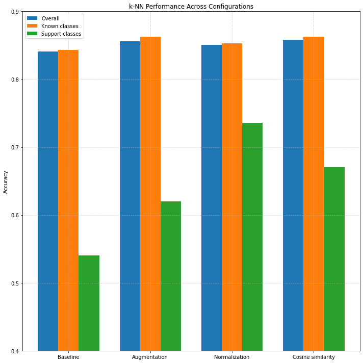
Figure 2: accuracy across configurations and class types.
Table IV and Figure 2 presents the results of a transfer learning approach in which a pretrained convolutional neural network (CNN) was used as a fixed feature extractor, followed by
nearest neighbor (NN) classification. Four experimental configurations were compared: a baseline (no augmentation or normalization), augmentation only, augmentation
with feature normalization, and augmentation with normalization and cosine similarity as the distance metric.
The baseline setup yielded an overall classification accuracy of 84.1%, with 84.3% accuracy on known classes and 54.0% on support classes.
Incorporating standard data augmentation techniques—such as random rotations, zooms, and brightness adjustments—led to a consistent improvement across all metrics,
increasing support class accuracy to 62.0% .
Further gains were observed when applying L2 normalization to the feature vectors, which projects them onto the unit hypersphere. This standardization improved
comparability between feature vectors and had a particularly notable effect on support class accuracy, which rose to 73.6%, the highest among all configurations.
This suggests that normalization is especially beneficial in few-shot scenarios, where model generalization is most challenging.
Finally, we tested cosine similarity as the distance metric in place of Euclidean distance. When used alongside augmentation and normalization, cosine similarity
produced the highest overall and known class accuracies (85.8% and 86.3%, respectively). However, support class performance slightly declined compared to the
normalized Euclidean setup, indicating that while cosine similarity improves general classification, it may be less effective for distinguishing among
underrepresented classes.
All evaluations used a consistent test set of 602 images, including 24 images from support classes. The total number of training images increased to 3107 in all
augmented scenarios due to the inclusion of synthetic variants.
In summary, the combination of data augmentation and L2 normalization was critical for enhancing performance in few-shot settings. Cosine similarity provided
marginal improvements in overall accuracy, though Euclidean distance remained preferable for support class discrimination.
Few-Shot identification: Transfer learning and metric learning: Prototypical Network
Dataset and feature extraction as described before. Here we calculate a prototype for each class, and the distance is measured for a query image to each prototype of each class. The prototype of a class with smallest distance becomes the predicted class.
Table V. Results for transfer learning and Prototypical Network
| Metrics | Value | |||
|---|---|---|---|---|
| Baseline | Augmentation | Normalization | Cosine similarity | |
| Overall accuracy | 0.714 | 0.728 | 0.761 | 0.728 |
| Known classes accuracy | 0.74 | 0.75 | 0.78 | 0.75 |
| Support classes accuracy | 0.46 | 0.51 | 0.61 | 0.54 |
| # images | 2947 | 3107 | 3107 | 3107 |
| The column "normalization" also includes augmentation. The column "cosine similarity" also include augmentation and feature normalization. | ||||
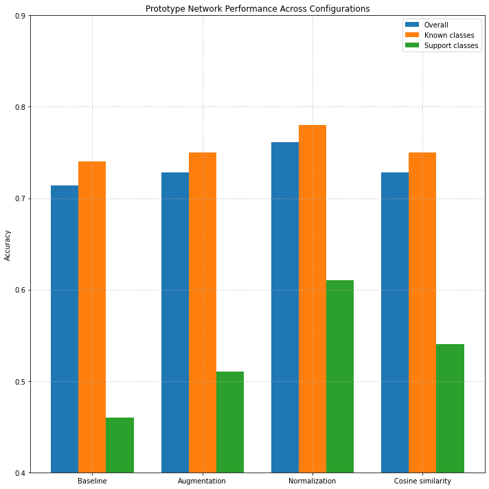
Figure 3: Accuracy across configurations and class types.
Table V presents the results of applying a prototypical network approach for classification using features extracted from a pretrained CNN. The table compares
four experimental conditions: a baseline configuration (no augmentation or normalization), augmentation only, augmentation with feature normalization, and augmentation
with normalization and cosine similarity as the distance metric.
In the baseline setting, the prototype classifier achieved an overall accuracy of 71.4%, with 74% accuracy on known classes and 46% accuracy on support classes.
Adding data augmentation yielded a modest improvement (figure 3), increasing overall accuracy to 72.8%, and slightly boosting both known class accuracy (75%) and support
class accuracy (51%). This reflects the expected benefit of data augmentation in improving generalization, particularly for underrepresented support classes.
Applying L2 normalization to the feature vectors, in addition to augmentation, led to the highest overall performance. This configuration yielded an overall accuracy
of 76.1%, a known class accuracy of 78%, and a notable increase in support class accuracy to 61%. The normalization step improves comparability of feature vectors
by projecting them onto the unit hypersphere, helping reduce the effect of scale variations in deep features.
Interestingly, using cosine similarity instead of Euclidean distance (while keeping augmentation and normalization) resulted in performance similar to the
augmentation-only setting: 72.8% overall accuracy and 54% support class accuracy. This suggests that while cosine similarity aligns well with normalized features,
it may not consistently outperform Euclidean distance for this particular task or dataset.
Few-Shot identification: Transfer learning and metric learning: Matching Network
Table VI presents the classification performance using a Matching Network approach built upon a fixed feature extractor from a pretrained convolutional neural network (CNN). The Matching Network employs a similarity-based nearest-neighbor mechanism where a query image is compared to all support set embeddings, and classification is performed using weighted soft voting over similarity scores. The results are shown across four experimental configurations: a baseline without augmentation or normalization, inclusion of standard data augmentation, feature normalization (which also includes augmentation), and finally a setup that uses both augmentation and normalization but applies cosine similarity as the distance metric.
Table VI. Results for transfer learning and Matching Network
| Metrics | Value | |||
|---|---|---|---|---|
| Baseline | Augmentation | Normalization | Cosine similarity | |
| Overall accuracy | 0.809 | 0.826 | 0.799 | 0.779 |
| Known classes accuracy | 0.81 | 0.84 | 0.81 | 0.78 |
| Support classes accuracy | 0.53 | 0.56 | 0.58 | 0.56 |
| # images | 2947 | 3107 | 3107 | 3107 |
| The column "normalization" also includes augmentation. The column "cosine similarity" also include augmentation and feature normalization. | ||||
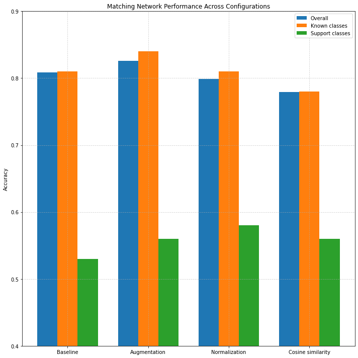
Figure 4: Accuracy across configurations and class types.
The baseline Matching Network achieved an overall accuracy of 80.9%, with 81% accuracy on known classes and 53% accuracy on the support (few-shot) classes. Incorporating data augmentation further increased performance across the board, yielding 82.6% overall accuracy, and support class accuracy of 56%. Interestingly, adding L2 normalization did not lead to further gains here (79.9% overall, 58% support), and using cosine similarity even resulted in a slight decline in performance (77.9% overall).
When compared to k-NN (as previously shown), Matching Networks achieve comparable support class performance in the baseline and augmentation configurations (e.g., 53% and 56% vs. 54% and 62% for k-NN), but lag in overall accuracy (k-NN reaches up to 85.6% under tuned settings). However, unlike k-NN, which is sensitive to class imbalance, Matching Networks apply a more structured attention mechanism, making them more adaptable under few-shot constraints [7].
Overall, Matching Networks offer better support class performance than Prototypical Networks in most configurations, and demonstrate robust generalization capabilities, particularly when paired with augmentation and normalization. Their performance confirms the benefit of leveraging instance-level similarities in low-data regimes, with less reliance on class centroids compared to the prototype approach.
Few-Shot identification: Transfer learning and Logistic Regression
Table VII presents the results of using logistic regression for classification in a transfer learning setting, where a fixed pretrained CNN is used to extract feature vectors for both query and support images. The classifier is evaluated under various configurations: baseline (no modifications), class weighting to address imbalance, data augmentation, feature normalization, and cosine similarity as a distance metric. Each setup explores the influence of these enhancements on both known and support class performance.
Table VII. Results for transfer learning and Logistic Regression
| Metrics | Value | ||||
|---|---|---|---|---|---|
| Baseline | Weighted classes | Augmentation | Normalization | Cosine similarity | |
| Overall accuracy | 0.932 | 0.949 | 0.947 | 0.889 | 0.882 |
| Known classes accuracy | 0.94 | 0.96 | 0.95 | 0.90 | 0.89 |
| Support classes accuracy | 0.68 | 0.70 | 0.76 | 0.68 | 0.66 |
| # images | 2947 | 2947 | 3107 | 3107 | 3107 |
| The column "normalization" also includes augmentation. The column "cosine similarity" also include augmentation and feature normalization. | |||||
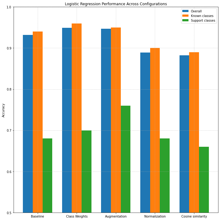
Figure 5: Accuracy across configurations and class types.
In the baseline configuration, logistic regression already achieves strong performance with an overall accuracy of 93.2% and a support class accuracy of 68%. Applying class weighting yields a modest improvement, increasing support class accuracy to 70%. Augmentation shows the most noticeable gain for the support set, pushing accuracy to 76% while maintaining high performance on known classes. However, applying normalization and cosine similarity slightly reduces performance on both known and support classes — suggesting that logistic regression performs best with raw feature magnitudes and standard Euclidean distance in this setup.
Compared to non-parametric methods like k-NN and Prototypical Networks, logistic regression exhibits significantly higher accuracy across all metrics. While k-NN achieved solid performance in earlier experiments, its sensitivity to class imbalance and local noise can limit its effectiveness in low-data scenarios. Prototypical Networks, while designed for few-shot tasks, assume compact and centered class distributions, which may not always align with real-world data, especially when classes exhibit intra-class variance. Matching Networks, which rely on pairwise similarity, performed well (support accuracy up to 58%) but fall short of logistic regression's parametric stability and superior generalization, particularly when augmented training data is available.
In summary, logistic regression serves as a strong baseline for few-shot classification with fixed CNN features. Its ability to generalize well from pretrained embeddings and its simplicity make it a valuable choice, especially when augmented data and balanced training strategies are applied.
Few-Shot identification: Transfer learning and Relation Network
Table VIII presents the results of applying a Relation Network-based approach to few-shot classification using a pretrained CNN feature extractor. The classifier computes relational similarity scores between query samples and averaged class prototypes, using a lightweight multi-layer perceptron (MLP) to assess similarity between embedding pairs. In the baseline configuration, the Relation Network achieves a strong overall accuracy of 92.5%, with 93% on known classes and an impressive 76% on support classes. This demonstrates that the model is particularly effective at generalizing to unseen classes in the few-shot regime when trained on raw CNN embeddings.
Table VIII. Results for transfer learning and Relation Network
| Metrics | Value | |||
|---|---|---|---|---|
| Baseline | Augmentation | Normalization | Cosine similarity | |
| Overall accuracy | 0.925 | 0.900 | 0.919 | 0.342 |
| Known classes accuracy | 0.93 | 0.91 | 0.93 | 0.37 |
| Support classes accuracy | 0.76 | 0.70 | 0.61 | 0.12 |
| # images | 2947 | 3107 | 3107 | 3107 |
| The column "normalization" also includes augmentation. The column "cosine similarity" also include augmentation and feature normalization. | ||||
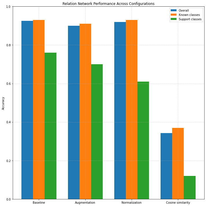
Figure 6: Accuracy across configurations and class types.
When data augmentation is introduced, overall accuracy slightly drops to 90%, and support class accuracy to 70%, suggesting that while augmentation may help in generalization for some models, it may introduce noise or variability that weakens relation-based similarity learning. Adding feature normalization helps recover some performance (91.9% overall), but interestingly, support class accuracy declines to 61%, indicating that centering or scaling features may hinder the learned similarity function’s robustness. When switching to cosine similarity in the final configuration, the model exhibits a drastic degradation in performance (overall accuracy drops to 34.2%, support class accuracy to just 12%). This sharp decline highlights that the MLP-based similarity function used in the relation network does not benefit from external similarity metrics like cosine distance, and instead performs best when relying on learned relationships between raw feature vectors.
Compared to the k-NN and Prototypical Network baselines, the Relation Network offers superior performance on support classes under the baseline
configuration (76% vs. 54% for k-NN and 46% for Prototypical Networks). This suggests that its learnable similarity function better captures non-linear
relationships between support and query features.
In contrast to Matching Networks, which achieved a maximum support class accuracy of 58%, the Relation Network shows higher few-shot generalization potential.
However, Matching Networks were more robust across various configurations and distance metrics. When compared with Logistic Regression, the Relation Network’s
baseline performance on support classes (76%) is competitive with the best logistic configuration (76%), though Logistic Regression generally showed more stable
performance across all settings, particularly under normalization and cosine similarity.
Discussion
This study explored various few-shot learning (FSL) methodologies leveraging a pretrained Convolutional Neural Network (CNN) as a fixed feature extractor for the classification of Morum species. Our methods encompassed non-parametric approaches (Nearest Neighbor, Prototypical Networks, and Matching Networks), a parametric approach (Logistic Regression), and a learnable metric-based method (Relation Networks). Each approach aimed to maximize generalization to new (support) classes with limited labeled instances.
Our results align with prior findings indicating that pretrained CNN features combined with straightforward classification methods can yield high performance even under severe data constraints [2, 8, 12]. Among the tested methods, logistic regression achieved the highest overall accuracy, reaching up to 94.9%, surpassing other approaches substantially. This outcome corroborates findings by Tian et al. (2020) [13] who demonstrated that linear classifiers on top of fixed CNN embeddings can rival sophisticated meta-learning approaches [13]. Furthermore, logistic regression showed robustness across configurations, particularly when combined with augmentation strategies, highlighting its practical applicability and stability under various preprocessing conditions, consistent with findings on robust LR estimation techniques [14, 17].
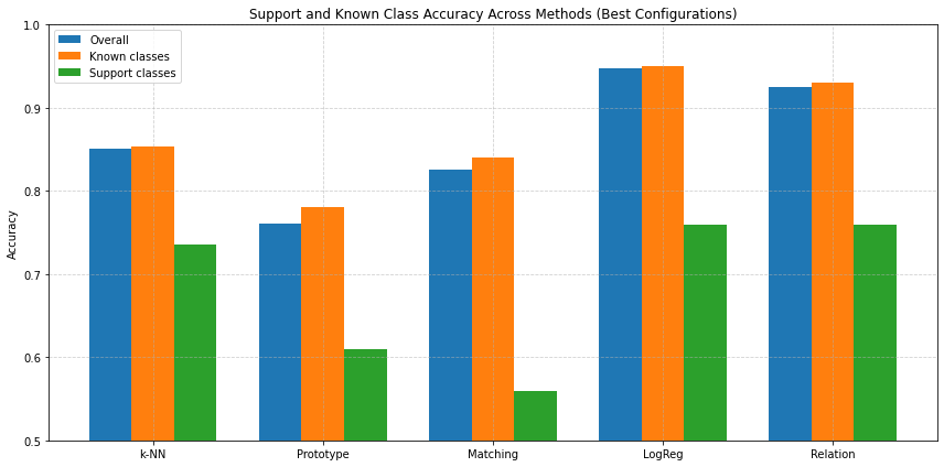
Figure 7: Overall, Known and Support Class Accuracy Across Methods (Best Configurations)
Nearest Neighbor classification provided a strong baseline, achieving an overall accuracy of approximately 85.8% under optimized conditions (augmentation and cosine similarity). Notably, its support class accuracy improved significantly with normalization (73.6%), which is consistent with literature emphasizing normalization's benefits for distance-based methods in high-dimensional feature spaces [2, 8]. However, k-NN's susceptibility to class imbalance was evident, limiting its effectiveness in distinguishing rare support classes compared to logistic regression and Relation Networks.
Prototypical Networks, while theoretically ideal for FSL due to their simplicity and inductive bias towards compact class clusters [5], achieved comparatively lower performance (76.1% peak accuracy) (figure 7). Their assumption of compact class centroids appears restrictive, especially given intra-class variance typical in biological data, echoing observations by Snell et al. (2017) on prototype methods' sensitivity to data distribution characteristics [5].
Matching Networks offered flexibility by leveraging instance-level similarity and soft-voting mechanisms. Their moderate performance (82.6% with augmentation) was generally robust but consistently trailed logistic regression (figure 7). The structured similarity calculation provided advantages over simple nearest neighbor methods in scenarios with class imbalance, aligning with Vinyals et al.’s findings on Matching Networks’ robustness under few-shot constraints [7].
Relation Networks performed exceptionally well on support classes (76% baseline accuracy), demonstrating superior capability in capturing nonlinear relationships between query and support features compared to Prototype and Matching Networks. However, performance sharply declined when feature normalization and cosine similarity were applied (34.2% overall accuracy), underscoring the MLP-based relation module’s sensitivity to feature preprocessing—a limitation noted by Sung et al. [11]. This observation suggests that Relation Networks are best utilized with raw, learned embeddings, as externally imposed similarity metrics hinder their learned metric function.
Our results further reinforce the critical role of data augmentation in enhancing model generalization in few-shot scenarios, particularly evident in logistic regression and k-NN performances. Conversely, the adverse effects observed with Relation Networks imply that augmentation strategies must be cautiously tailored to the chosen method.
The success of all evaluated methods hinges on the quality of the features extracted from the CNN pretrained specifically on Morum species. The high validation accuracy (~94%) achieved by this base model (Table II, Table III) indicates that its penultimate layer captured discriminative morphological features relevant to this genus. This aligns with established principles of transfer learning, where representations learned on large, related datasets prove beneficial for downstream tasks with limited data [15, 16]. Our results extend findings from studies using general datasets like ImageNet [e.g., 8, 13], demonstrating the power of domain-specific pretraining for specialized tasks like fine-grained species identification. The effectiveness of these fixed features across diverse classifiers (parametric, non-parametric, metric-based) further validates their utility in this FSL scenario.
An observation is the variable impact of L2 normalization. While significantly boosting distance-based methods like k-NN and Prototypical Networks (likely by emphasizing angular separation over magnitude in the feature space ), it offered no benefit or was even detrimental to Logistic Regression and Relation Networks. This suggests that for this Morum feature space, the raw feature magnitudes captured information valuable for linear separation (LR) and the learned similarity metric (RN), which was potentially obscured by normalization. This highlights that optimal post-processing is highly dependent on the interplay between the feature space characteristics and the downstream classification algorithm.
However, the study has limitations. The findings are specific to the Morum dataset and the single pretrained CNN architecture used; generalization to other taxa or different base models requires further investigation. The number of support classes and the number of shots (minimum 6 images) are relatively small, though representative of real-world data scarcity for rare species. We only utilized features from the penultimate layer and did not explore feature fusion or fine-tuning the extractor. Furthermore, we focused on transfer learning baselines and did not directly compare against state-of-the-art meta-learning algorithms, which might offer different trade-offs.
The choice between classifier simplicity (such as Logistic Regression) and complexity (like Relation Networks) involves critical trade-offs for practical deployment. Logistic Regression offers computational efficiency, interpretability, and robustness to limited data, making it ideal for resource-constrained environments or real-time applications, so this option is preferred for an implementation in the IdentifyShell.org application. Conversely, Relation Networks, despite their higher complexity and computational demands, can model intricate non-linear relationships and may yield superior performance on challenging, fine-grained tasks, a method which will be used in future research.
In conclusion, this comparative study of FSL methods highlights logistic regression’s efficacy, practical simplicity, and robustness, making it particularly suited to real-world biological classification tasks where data is scarce and class distributions imbalanced. Relation Networks offer compelling alternatives when nonlinear relationships are pronounced, provided careful attention to data preprocessing.
Expanding the study to other taxonomic groups and datasets to assess the generalizability of these findings is an important next step. The effectiveness of pretrained CNN features likely hinges on morphological similarity and taxonomic proximity, meaning closely related species might benefit similarly, while more distant taxa could experience reduced performance due to differing morphological characteristics. Future research should thus investigate diverse taxonomic groups to assess the robustness and limits of these FSL approaches across other taxa of the Mollusca phylum. In other words, the purpose of this study was to identify promising CNN-based pipelines for FSL to be used on many nodes in our hierarchical CNN for Mollusca.
Investigating features from different network layers or employing feature selection might yield further improvements. Exploring the potential benefits of fine-tuning the feature extractor, rather than keeping it fixed, warrants investigation, though it risks overfitting with limited support data. Comparing these transfer learning baselines against established meta-learning algorithms (e.g., MAML, Reptile) on this dataset would provide valuable context. Finally, delving deeper into the reasons behind the performance degradation of Relation Networks with standard post-processing techniques could offer insights into the behaviour of learned similarity metrics.
Conclusion
In conclusion, this study demonstrates the successful application of transfer learning-based few-shot learning for identifying rare Morum species using features from a domain-specific pretrained CNN. Logistic Regression and Relation Networks (baseline) provided the highest accuracy for identifying novel support classes, achieving 76% accuracy. k-Nearest Neighbors also performed strongly when combined with L2 feature normalization (73.6% support accuracy). The results highlight that while powerful pretrained features are crucial, the downstream choice of classifier and feature post-processing significantly influences performance in the few-shot regime, with interactions that may differ from those observed on standard benchmarks. These findings underscore the potential of relatively simple, well-configured transfer learning approaches for tackling real-world biological identification challenges characterized by data scarcity.
References
- [1] Liu, Y. et al. Few-Shot Image Classification: Current Status and Research Trends.. Electronics 2022, 11, 1752 (2022)
- [2] Wang, Y. et al. SimpleShot: Revisiting Nearest-Neighbor Classification for Few-Shot Learning. arXiv:1911.04623 (2019)
- [3] Hu, S.X. et al. Pushing the Limits of Simple Pipelines for Few-Shot Learning: External Data and Fine-Tuning Make a Difference. IEEE/CVF Conference on Computer Vision and Pattern Recognition (CVPR), pp. 9058-9067 (2022)
- [4] Katageri, R. et al. Transfer Learning in Computer Vision. International Journal of Scientific Research and Engineering Development Volume 6 Issue 4 (2023)
- [5] Snell, J. et al. Prototypical networks for few-shot learning. JProceedings of the 31st International Conference on Neural Information Processing Systems, pp. 4080-4090 (2017)
- [6] Kornblith, S. et al. Do Better ImageNet Models Transfer Better?. Proceedings of the IEEE/CVF Conference on Computer Vision and Pattern Recognition (CVPR), 2661–2671 (2019)
- [7] Vinyals, O. et al. Matching Networks for One Shot Learning. Advances in Neural Information Processing Systems, 29 (2016)
- [8] Chen, W.-Y. et al. A Closer Look at Few-shot Classification. International Conference on Learning Representations (ICLR) (2019)
- [9] Donahue, J. et al. DeCAF: A Deep Convolutional Activation Feature for Generic Visual Recognition. International Conference on Machine Learning (ICML) (2014)
- [10] Sun, Q. et al. Meta-Transfer Learning for Few-Shot Learning. IEEE Conference on Computer Vision and Pattern Recognition (CVPR) (2020)
- [11] Sung, F. et al. Learning to Compare: Relation Network for Few-Shot Learning. IEEE Conference on Computer Vision and Pattern Recognition (CVPR), (2018)
- [12] Dhillon, G. et al. A Baseline for Few-Shot Image Classification. International Conference on Learning Representations (ICLR) (2020)
- [13] Tian, Y., et al. Rethinking Few-Shot Image Classification: A Good Embedding Is All You Need?. European Conference on Computer Vision (ECCV), pp. 266–282 (2020)
- [14] Bishop, C.M. Pattern Recognition and Machine Learning. Information Science and Statistics, ISSN 1613-9011 (2006)
- [15] Oquab, M. et al. Learning and transferring mid-level image representations using convolutional neural networks. IEEE Conference on Computer Vision and Pattern Recognition, Columbus, OH, USA, 2014, pp. 1717-1724 (2014)
- [16] He, K. et al. Deep residual learning for image recognition. Proceedings of the IEEE Conference on Computer Vision and Pattern Recognition pp. 770-778 (2016)
- [17] Rousseeuw, P. J., & Christmann, A. Robustness against separation and outliers in logistic regression. Computational Statistics & Data Analysis,1 43(3), 315-332 (2003)