Deep Learning Morphology in Integrative Phylogenetics: Insights from genus Hastula (Terebridae)
Published on: August 2025
Abstract
Shell morphology has long been used to classify gastropods, yet it is prone to convergence and often poorly reflects evolutionary history. Molecular phylogenies have provided more reliable frameworks, but integrating morphological and molecular evidence remains a central challenge in systematics. Here we use the sand-dwelling auger snails of the genus Hastula (family Terebridae) as a case study to evaluate the phylogenetic signal of morphology extracted with convolutional neural networks (CNNs). A CNN model trained on 3,204 shell images representing 23 species achieved high performance in species-level identification (93% validation accuracy). Feature vectors from the network were used to compute pairwise cosine distances, construct similarity matrices, and infer morphological trees by hierarchical clustering and neighbor-joining with bootstrapping. These analyses revealed coherent morphological clusters, such as Hastula matheroniana + H. strigilata and H. albula + H. solida + H. hectica, while taxa with fewer images (H. salleana, H. rufopunctata) showed reduced performance and isolated placement.
Comparison with a multilocus phylogeny (12S, 16S, COI, 28S) of 15 Hastula species revealed both overlaps and conflicts. While some associations were recovered in both datasets, including H. matheroniana + H. penicillata, other relationships differed, notably H. lanceata + H. strigilata (strongly supported molecularly but absent in CNN-based trees). Quantitative metrics confirmed limited congruence: the Robinson–Foulds distance was 16/18 (normalized RF = 0.889), and the Mantel test indicated only a weak, non-significant correlation between molecular and morphological distances (r = 0.228, p = 0.225).
These results demonstrate that CNN-derived features capture biologically meaningful morphological signal but only partially align with evolutionary history. As in other gastropods, shell convergence likely explains much of the discordance. We argue that CNN-based morphology is best deployed within integrative, total-evidence frameworks that combine DNA, morphology, and ecology to resolve evolutionary relationships in Terebridae.
Introduction
The use of shell morphology has historically been the primary basis for classifying gastropods, including the sand-dwelling auger snails (family Terebridae). While shells provide abundant and readily accessible characters, they are also prone to convergence and homoplasy. Similar forms often evolve independently under shared ecological pressures, such as burrowing lifestyle or sediment type, leading to morphological groupings that do not always reflect evolutionary history [1, 2]. As a result, morphology-only classifications of gastropods frequently conflict with molecular evidence, and it is now widely accepted that integrative approaches combining DNA and morphology are essential for robust systematics [1, 2] .
Molecular phylogenetics has revolutionized the classification of Conoidea, the diverse superfamily that includes cone snails (Conidae), auger snails (Terebridae), and their relatives. Early shell- and radula-based systems often grouped unrelated taxa, while DNA evidence has consistently revealed that many traditional genera were polyphyletic or paraphyletic [4]. Within Terebridae specifically, the first broad molecular phylogeny [3] confirmed the family’s monophyly and identified five major clades (A–E), each corresponding to lineages with distinct evolutionary histories. Among these, Hastula (Clade D) emerged as a coherent and well-supported genus, validating its traditional recognition on the basis of its smooth, glossy, and elongate shells. It is also demonstrated [3] that anatomical traits such as the venom apparatus had been lost independently in multiple terebrid lineages, underscoring the need for molecular evidence to reconstruct evolutionary history reliably [3].
Subsequent work expanded and refined this framework. Macroevolutionary analyses across Terebridae [5] revealed that diversification was more strongly associated with environmental factors than with the gain or loss of the venom gland. This highlighted the role of ecology in shaping terebrid diversity and suggested that shell morphology may often capture ecological adaptation rather than phylogenetic signal. Fedosov et al. (2020) [6] integrated multilocus DNA data with shell and anatomical traits in a comprehensive revision of the family. They proposed a three-subfamily classification (Pellifroniinae, Pervicaciinae, Terebrinae) and formally redefined genera to align taxonomy with molecular clades. Hastula was retained as a valid genus within Terebrinae, encompassing a distinct radiation of venomous, shallow-water sand-dwelling auger snails. Although morphologically cohesive, Fedosov et al. also noted substantial substructure within Hastula and emphasized the prevalence of convergence across the family, advocating for DNA-based diagnoses coupled with detailed morphological descriptions [6].
In parallel with these molecular advances, new computational tools have made it possible to revisit morphological data in novel ways. Deep learning, and particularly convolutional neural networks (CNNs), can extract complex quantitative features from shell images, capturing aspects of morphology that may be difficult to describe using traditional character coding. Recent proof-of-concept studies have shown that CNN-derived morphological embeddings can be used to construct distance matrices and even phylogenetic trees, providing a new source of automated, high-dimensional morphological data [7]. While such morphology-derived trees often differ from DNA-based topologies, they offer a complementary perspective and can be integrated into total-evidence frameworks that combine molecules, morphology, and fossils [2, 6, 7].
Here we present a case study of Hastula that applies CNN-based morphology alongside multilocus molecular phylogenetics. Building on earlier investigations in Oxymeris and other terebrids, we evaluate the performance of CNNs for species-level identification, examine whether CNN-derived feature spaces capture morphological affinities among species, and compare these morphological hypotheses with DNA-based phylogenies. This approach allows us to assess both the strengths and limitations of CNN-based morphology in reflecting evolutionary history and to explore how such methods can be integrated into the ongoing effort to align auger snail taxonomy with phylogeny.
Methods
Data Acquisition
Shell images were collected from many online resources, from specialized websites on shell collecting to institutes and universities. One of the largest collections of shell images is available on GBIF. Also online marketplace such as ebay contain a large collection of images. Other large shell image collections are available at , Malacopics, Femorale and Thelsica. A shell dataset created for AI is available [8].
Some online resources have facilities to download images, but most websites require a specialized webscraper. Scrapy , an open source and collaborative framework for extracting the data from websites, is used to create a custom webscraper to extract images and their scientific names. All data was stored in a MySQL database before further processing was performed.
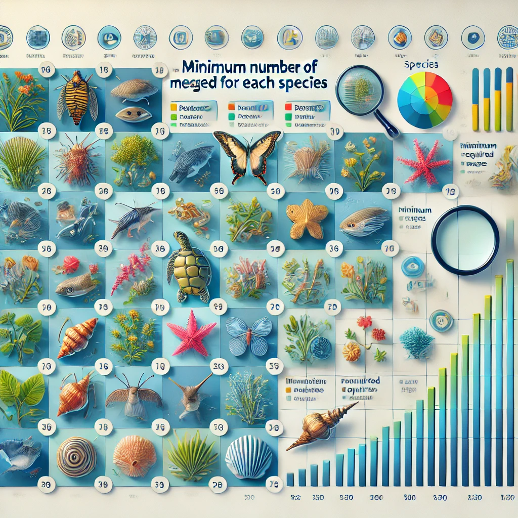
The dataset for the Hastula CNN model comprises 3204 shell images representing 23 Hastula species (see table II). There are 104 species in the genus Hastula (WoRMS or MolluscaBase), but not enough images were found for 81 species. Species with less than 25 images were removed (see Minimum number of images needed for each species).
All sequences were retrieved from https://www.ncbi.nlm.nih.gov/gene/ using search expression "Terebridae"[Organism] OR Terebridae[All Fields]. A total of 3398 entries were retrieved and stored locally in a BioSQL database. These data were cross checked with MolluscaBase/WoRMS.
The sequences selected for this report are the ribosomal DNA , mitochondrial 12S, 16S and nuclear 28S and the mitochondrial Cox1 gene that have a valid MolluscaBase name. The publications with the source of most sequences are those by Holford et al. (2009) [3] and Modica et al. (2020) [5]
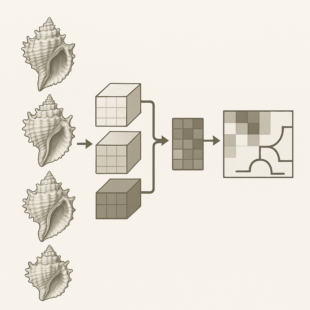
Image Pre-processing
All names were checked against WoRMS or MolluscaBase for their validity. Names that
were not found in WoRMS/MolluscaBase were excluded for further processing. While a large part of this data
quality step was automated, a manual verification (time-consuming) step was also included. In addition to text-based quality control, both
automated and manual preprocessing steps were applied to the images.
When an image contained multiple shells, we applied thresholding to binarize the background and then used
contour detection to locate each shell’s outline, cropping out each detected contour as an individual image.
The background was replaced with a uniform black background. A square image was made by padding with a black background. All shells were
resized (400 x 400 px). A final visual selection was made before producing
the final image dataset. Overall, 10-20% of the images were removed for various reasons (when other objects
were visible in the picture such as hands, habitat, text, etc.).
Hardware
An HP Omen 30L GT13 was used for training the model. It contains a Intel(R) Core(TM) i9-10850K CPU @ 3.60GHz processor, with 64GB RAM, Nvidia GeForce RTX 3080 10GB.
Model Training
For this study, Python (version 3.10.12) was used. The EffiecientNetV2B2 pre-trained models were used. (see Identifying Shells using Convolutional Neural Networks: Data Collection and Model Selection) Table 2 lists the hyperparameters. The models were trained using a batch size of 64 samples, and the number of epochs used was 100. The learning process was initiated with an initial learning rate of 0.0005 and the Adam optimiser was utilised for efficient weight updates. Two callbacks were used, one to monitor the validation loss and decreasing the learning rate , a second callback for early stopping. Both callbacks were applied to prevent the model from over-fitting. Fine-tuning the model was performed as described before. The top 3 layers of the model were unfrozen.
Table I. Hyperparameters
| Hyperparameter | Value | Comments |
|---|---|---|
| Batch Size | 64 | |
| Epochs | 100 | The number of epochs determines how many times the entire training dataset is passed through the model. Because early-stopping is used, often less than 100 epochs were needed. The current model ran for 30 epochs |
| Optimizer | Adam | The optimizer determines the algorithm used to update model weights during training. |
| Learning Rate | 0.0005 |
The validation loss was monitored and adjusted
reduce_lr = keras.callbacks.ReduceLROnPlateau(monitor='val_loss', factor=0.1, patience=3, min_lr=1e-6) |
| Loss | Categorical Cross-entropy | |
| Regularization | 0.0001 |
Evaluation Metrics
The evaluation of the performance of the CNN models was carried out by using standard metrics for
classification: accuracy, precision, recall, and F1 score,
which are defined by [9] in terms of the number of FP (false positives); TP (true
positives); TN (true negatives); and FN (false negatives) as follows:
Feature vectors from the the penultimate layer of the trained Hastula CNN model
To analyze the internal representations learned by the Hastula CNN model, we extracted high-dimensional
feature vectors from the penultimate layer of the trained network.
These embeddings capture rich semantic information about each image while abstracting away from pixel-level
details. The model was implemented and trained using TensorFlow, and feature vectors were obtained using Keras’ Model subclassing, where a truncated version of the network
outputs activations from the final convolutional or dense layer
prior to classification. Each image in the dataset was passed through the network in inference mode, and the
resulting feature vector (1408 dimensions) was stored for further analysis.
To quantify similarity between images, we computed pairwise cosine similarity between feature vectors.
For each image , compute similarity to all other images in the same class:
and are the feature vectors (or embeddings) corresponding to image and image , respectively. These are extracted from the penultimate layer of the trained CNN and represent the model's internal encoding of visual characteristics in a high-dimensional space.
Cosine similarity measures the cosine of the angle between two vectors in the embedding space, and is particularly well-suited for high-dimensional data where the magnitude of the vectors is less informative than their direction. It was calculated using the sklearn.metrics.pairwise.cosine_similarity function from scikit-learn. Cosine distance (1 - similarity) was used when required for clustering, outlier detection, or visualization purposes. This approach allowed us to evaluate both intra-class cohesion and inter-class separation based on the learned feature representations, providing a model-centric view of image similarity beyond what can be captured by raw pixel comparisons.
CNN NJ analysis
The CNN-based morphological tree was constructed by aggregating deep visual features extracted from a trained convolutional neural network model. First, species-level representations were obtained by averaging the feature vectors of individual images per species, resulting in a feature matrix of shape (23 species × F features). To account for variation and assess cluster robustness, we applied a non-parametric bootstrapping strategy: for each of 500 replicates, the feature dimensions (columns) were resampled with replacement, and cosine distances were computed between species. These distance matrices were converted into phylogenetic distance matrices and used to infer neighbor-joining (NJ) trees via the DendroPy library.
Across all replicates, bipartitions (internal nodes) were encoded and tallied to compute their frequency of occurrence. For each unique bipartition present in ≥50% of replicates, a majority-rule consensus tree was constructed. Branch lengths were set to the mean length observed for each split across replicates, and bootstrap support values were annotated as the percentage of trees in which each bipartition appeared. To ensure consistency with the molecular dataset, either all 23 species or a subset of 8 species overlapping with the sequence-based tree were included, depending on the analysis. The resulting consensus trees were exported in Newick format and visualized using ETE3, with species labels, support values, and branch lengths graphically rendered for interpretability.
Comparing morphological trees
To evaluate the impact of tree construction method on species relationships inferred from morphological features, we compared a Neighbor-Joining (NJ) tree with a hierarchical clustering tree constructed using the average linkage (UPGMA) algorithm. Both trees were derived from the same CNN-based morphological distance matrix computed from species-level averaged feature vectors. The NJ tree was inferred using the nj() function from the scikit-bio library, while the UPGMA tree was generated via the scipy.cluster.hierarchy.linkage() function with the 'average' method applied to a condensed distance matrix. To assess topological differences, we computed the Robinson–Foulds (RF) distance using ete3, which quantifies the number of bipartitions that differ between two unrooted trees. This metric provides an objective measure of topological similarity between the trees, independent of branch lengths.
Hastula phylogenetic trees
To extract the phylogenetic relationships among species of the genus Hastula, we pruned the full Terebridae species tree to retain only terminal taxa of the genus Hastula. The tree was previously inferred from concatenated DNA sequence alignments using a species tree approach, and encoded in extended Newick format with metadata annotations. The pruning and visualization were conducted using the ete3 toolkit in Python. Branch lengths were preserved from the original tree, and internal support values were extracted from the pp1 metadata tag embedded in node labels. These posterior probabilities represent support from gene-tree reconciliation and were annotated below each internal node in the resulting subtree.
Comparing morphological and molecular tree
To quantify topological similarity between the morphology-based and molecular phylogenies, we again computed the Robinson–Foulds (RF) distance using the ete3 library in Python. Prior to comparison, we ensured that both trees contained identical sets of taxa by pruning and standardizing leaf names. The RF distance was computed in unrooted mode, and normalized by the maximum possible RF distance given the shared set of taxa (see also 'Comparing morphological trees'). This normalization yields a tree similarity score between 0 (completely different) and 1 (identical).
To assess the correspondence between the molecular and CNN-derived morphological distance matrices, we performed a Mantel test using the skbio Python package. The test evaluates the correlation between two symmetric distance matrices of equal dimensions using Pearson’s correlation coefficient, with 999 permutations to assess statistical significance. The molecular distance matrix was derived from distances on the phylogeny inferred from sequence data, while the morphological matrix was based on pairwise cosine distances computed from species-level CNN feature vectors. Both matrices were aligned to ensure the same taxon ordering, symmetrized to enforce strict matrix symmetry, and formatted as required by the Mantel test.
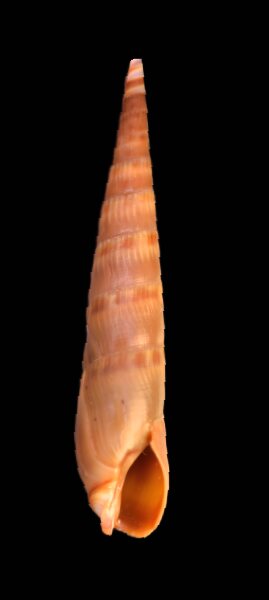
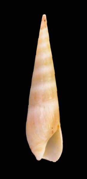
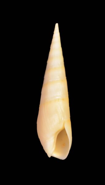
Figure 1: Representative images of Hastula species used in this study. Examples of shell images from the dataset, illustrating the morphological diversity within the genus Hastula. The CNN was trained to distinguish species based on visual features such as shell shape, color patterns, and ornamentation. From left to right: Hastula cinerea, H. hectica, and H. aciculina.
Results
CNN model
The CNN model trained for Hastula species identification achieved good classification performance, as reflected in both overall metrics and per-species results. The final training accuracy reached 98%, with a validation accuracy of 93%, indicating acceptable generalization to unseen data. Although some degree of overfitting is evident — given that validation accuracy is lower than training accuracy — the corresponding loss values (training loss: 0.196, validation loss: 0.297) remain well within acceptable ranges, suggesting stable training dynamics and effective convergence.
A detailed breakdown of performance by species is provided in Table II, which lists recall, precision, and F1-score for each of the 23 Hastula species. Note that H. stylata (Hinds, 1844) is now a synonym of H. cinerea (Born, 1778), but this change was recent (MolluscaBase). In this analysis we consider H. stylata as a separate class/species.
Table II. Species-level classification performance of the CNN model
| Species | # images | Recall | Precision | F1 |
|---|---|---|---|---|
| Hastula aciculina (Lamarck, 1822) | 227 | 0.955 | 0.955 | 0.955 |
| Hastula alboflava Bratcher, 1988 | 105 | 1.000 | 1.000 | 1.000 |
| Hastula albula (Menke, 1843) | 236 | 0.878 | 0.973 | 0.923 |
| Hastula bacillus (Deshayes, 1859) | 104 | 1.000 | 0.828 | 0.906 |
| Hastula cinerea (Born, 1778) | 323 | 0.855 | 0.908 | 0.881 |
| Hastula cuspidata (Hinds, 1844) | 81 | 0.889 | 0.762 | 0.821 |
| Hastula escondida (Terryn, 2006) | 74 | 0.944 | 0.944 | 0.944 |
| Hastula exacuminata Sacco, 1891 | 53 | 0.867 | 0.813 | 0.839 |
| Hastula hastata (Gmelin, 1791) | 131 | 0.958 | 0.920 | 0.939 |
| Hastula hectica (Linnaeus, 1758) | 184 | 0.912 | 1.000 | 0.954 |
| Hastula inconstans (Hinds, 1844) | 78 | 1.000 | 0.900 | 0.947 |
| Hastula lanceata (Linnaeus, 1767) | 337 | 1.000 | 1.000 | 1.000 |
| Hastula leloeuffi Bouchet, 1983 | 70 | 1.000 | 1.000 | 1.000 |
| Hastula lepida (Hinds, 1844) | 148 | 1.000 | 1.000 | 1.000 |
| Hastula maryleeae R. D. Burch, 1965 | 105 | 0.737 | 0.875 | 0.800 |
| Hastula matheroniana (Deshayes, 1859) | 208 | 0.947 | 0.947 | 0.947 |
| Hastula penicillata (Hinds, 1844) | 109 | 0.923 | 0.923 | 0.923 |
| Hastula raphanula (Lamarck, 1822) | 146 | 1.000 | 0.957 | 0.978 |
| Hastula rufopunctata (E. A. Smith, 1877) | 38 | 0.818 | 0.750 | 0.783 |
| Hastula salleana (Deshayes, 1859) | 40 | 0.500 | 0.500 | 0.500 |
| Hastula solida (Deshayes, 1859) | 106 | 1.000 | 0.950 | 0.974 |
| Hastula strigilata (Linnaeus, 1758) | 189 | 0.905 | 0.927 | 0.916 |
| Hastula stylata (Hinds, 1844) | 112 | 0.867 | 0.867 | 0.867 |
| This table provides a detailed breakdown of the model's classification performance for each of the 23 Hastula species included in the study. # images indicates the total number of images used for each species. Recall (Sensitivity) measures the model's ability to correctly identify all images of a given species. Precision measures the proportion of correct identifications among all images assigned to a species. The F1-score is the harmonic mean of precision and recall, providing a single metric for overall accuracy per species. Values approaching 1.0 indicate high performance. | ||||
Species-level performance metrics are summarized in Table II. For most taxa, recall, precision, and F1-scores were consistently high, with several species such as H. alboflava, H. lanceata, H. leloeuffi, and H. lepida achieving perfect scores across all three metrics. Other common species with larger sample sizes, such as H. cinerea and H. strigilata, also showed robust classification (F1-scores 0.881 and 0.916, respectively), though with slightly lower recall, reflecting some residual misclassification.
A few species with smaller sample sizes displayed reduced performance. For instance, H. salleana (n = 40) was the most challenging to classify, with balanced but low recall and precision (0.50 each), indicating frequent confusion with morphologically similar taxa. Similarly, H. rufopunctata (n = 38) yielded lower precision (0.750), suggesting that images of other species were occasionally misclassified as H. rufopunctata. In contrast, H. hectica and H. solida showed near-perfect identification, with F1-scores above 0.95 despite moderate sample sizes.
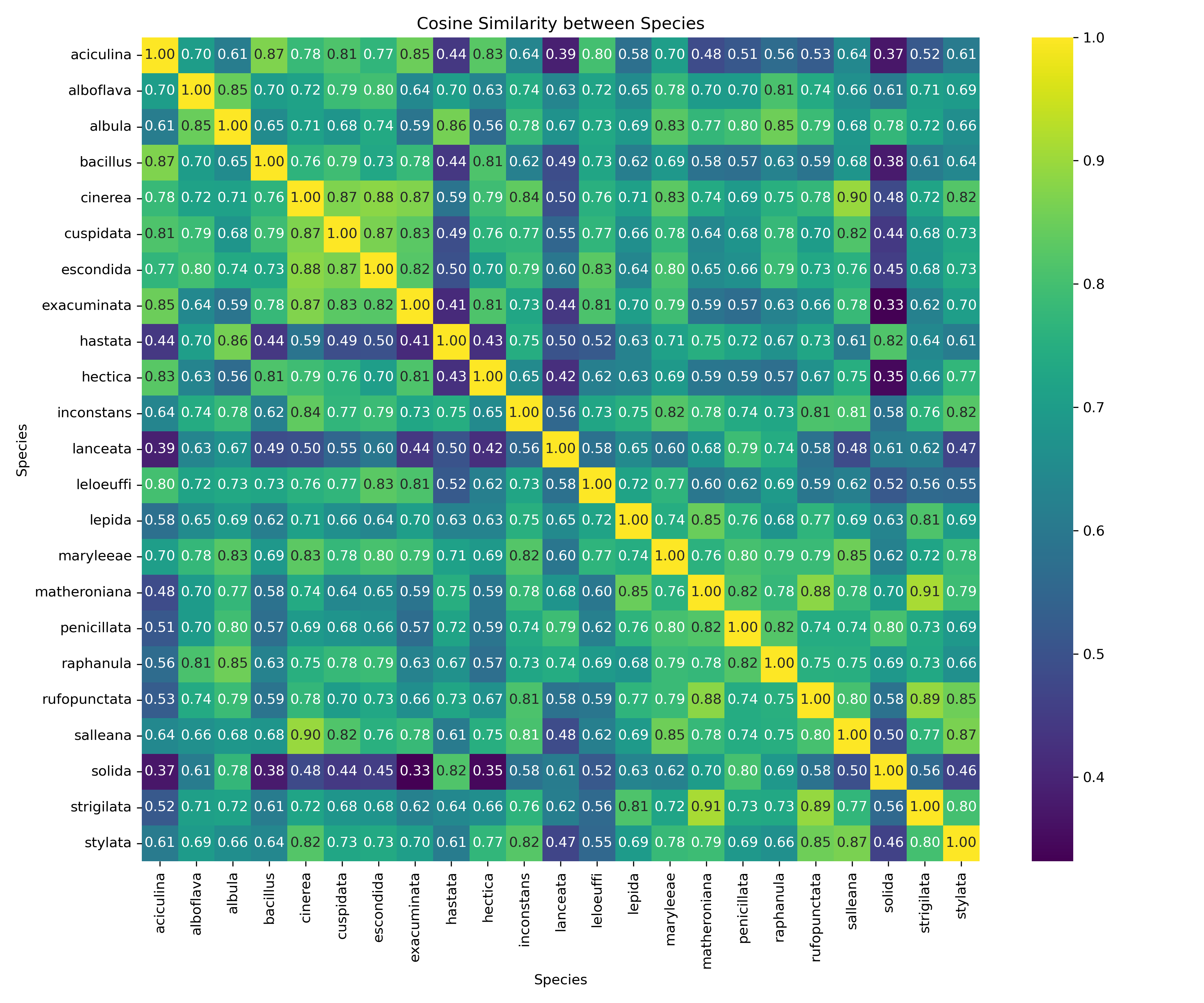
Figure 2. Pairwise cosine similarity matrix of Hastula species based on CNN feature vectors. This matrix quantifies the morphological similarity between species as learned by the CNN. Each cell contains the cosine similarity value between the averaged feature vectors of two species. Values range from 0 to 1, where 1 (along the diagonal) represents perfect self-similarity. Higher off-diagonal values (e.g., > 0.80) indicate that the model perceives two species as very similar in shell morphology, while lower values (e.g., < 0.40) indicate high distinctiveness in the learned feature space.
To better understand the relationships underlying these performance patterns, we next examined the feature-space similarity between species using CNN embeddings.
In addition to classification metrics, the learned feature representations were examined by computing pairwise cosine similarity between the averaged CNN feature vectors of each Hastula species (Figure 2). The resulting similarity matrix provides insights into how the model perceives morphological relationships across species.
Off-diagonal values ranged from as low as 0.33 to as high as 0.91, reflecting a spectrum from highly distinctive to closely overlapping morphologies. Several clusters of high similarity (cosine similarity > 0.80) were observed, suggesting that the CNN identifies morphological affinities between certain species pairs. Species such as H. salleana and H. rufopunctata displayed moderate to low similarity with most other taxa (values < 0.50 in several comparisons), highlighting their morphological distinctiveness in the feature space. This observation is in line with their reduced per-species classification performance, suggesting that limited training samples combined with unique morphologies posed challenges for the model.
Overall, the similarity matrix illustrates that the CNN not only learns to discriminate species but also captures meaningful morphological structure within the genus. Groups of species with high pairwise similarity likely reflect genuine phenotypic overlap, while low-similarity taxa represent distinct morphotypes. This provides further evidence that CNN-derived features can be used not only for accurate classification but also for quantitative assessments of morphological relatedness across species.
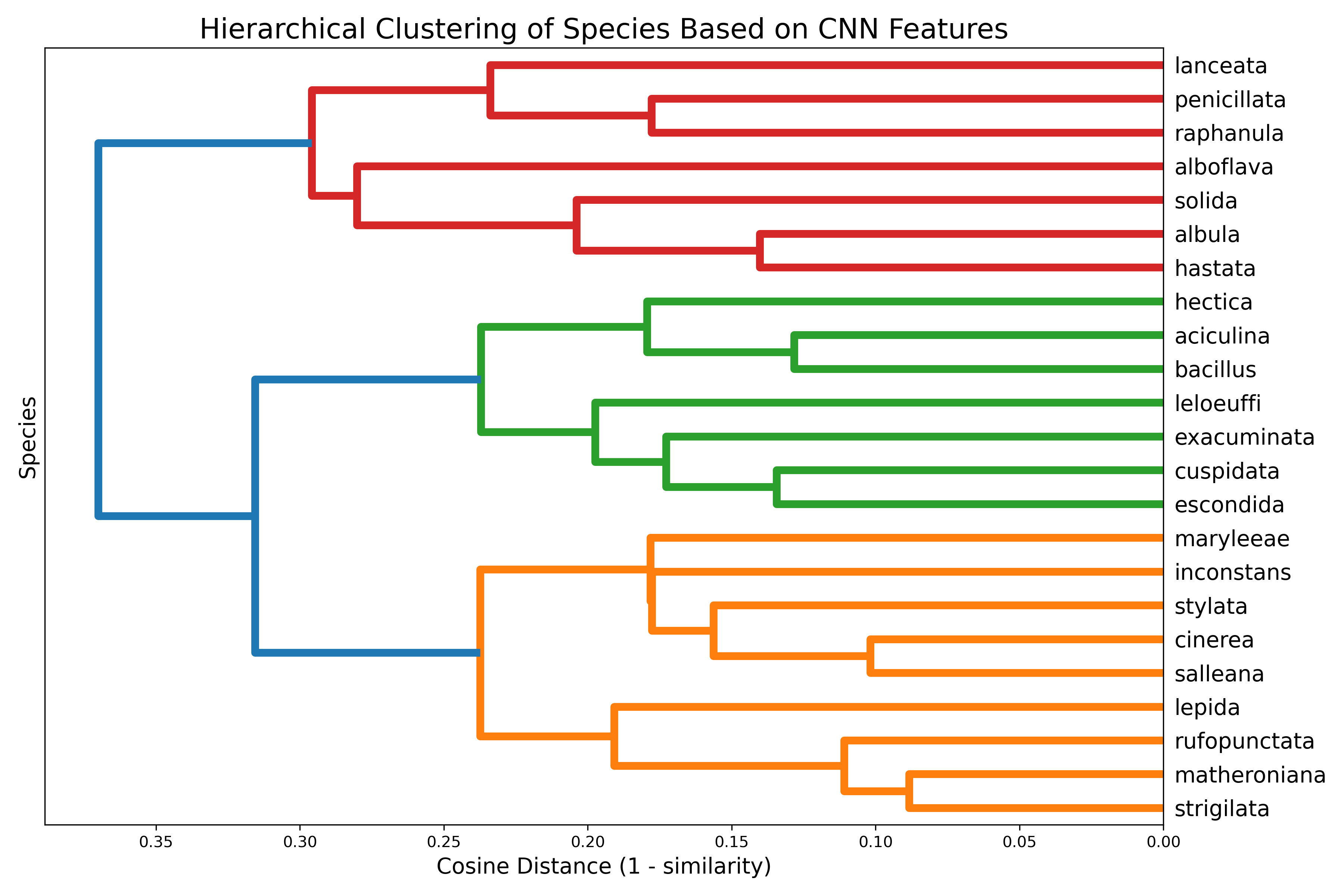
Figure 3: Hierarchical clustering of Hastula species based on CNN-derived morphological distances. This dendrogram illustrates the phenetic relationships among the 23 Hastula species based on their visual similarity. The tree was constructed using the Unweighted Pair Group Method with Arithmetic Mean (UPGMA) algorithm applied to a matrix of pairwise cosine distances (calculated as 1 - cosine similarity) between the species-averaged feature vectors. Species that cluster together with shorter branch heights are interpreted by the CNN as being more morphologically similar.
To further explore morphological relationships among the studied taxa, hierarchical clustering was performed on the CNN-derived feature vectors, using cosine distance as a measure of dissimilarity (Figure 3). The resulting dendrogram provides a phenetic representation of interspecific similarity as perceived by the model.
Hierarchical clustering of CNN features (Figure 3) revealed three major clusters of Hastula. The first (red) contained seven species including H. lanceata, H. penicillata, and H. solida. The second (green) grouped taxa such as H. hectica, H. aciculina, and H. leloeuffi. The third (orange) was the most diverse, encompassing H. matheroniana, H. strigilata, H. cinerea, and others. Within this cluster, H. matheroniana and H. strigilata formed a close pair, while more distinctive species such as H. salleana and H. rufopunctata occupied more isolated positions.
- The first cluster (red) contained seven species (H. lanceata, H. penicillata, H. raphanula, H. alboflava, H. solida, H. albula, H. hastata), several of which also achieved very high classification scores (Table II). Their short branch lengths indicate high similarity in CNN-derived features.
- The second cluster (green) grouped together H. hectica, H. aciculina, H. bacillus, H. leloeuffi, H. exacuminata, H. cuspidata, and H. escondida. This cluster represents a second morphologically coherent group as recognized by the CNN.
- The third cluster (orange) was the largest and most internally diverse, comprising nine species (H. maryleeae, H. inconstans, H. stylata, H. cinerea, H. salleana, H. lepida, H. rufopunctata, H. matheroniana, and H. strigilata). This group contained both tightly paired taxa (e.g., H. matheroniana and H. strigilata) as well as more isolated species (H. salleana, H. rufopunctata), reflecting both similarity and distinctiveness within this cluster. It includes H. cinerea and synonym H. stylata.

Figure 4: Neighbor-joining consensus tree of Hastula species based on CNN morphological features. Phylogenetic hypothesis for Hastula based solely on CNN-derived morphological data. This is a 50% majority-rule consensus tree from 500 bootstrap replicates. The tree was inferred using the neighbor-joining (NJ) algorithm from the cosine distance matrix. Numbers at the nodes represent bootstrap support percentages, indicating the frequency at which a given clade appeared in the replicates. Branch lengths are proportional to the mean cosine distance between nodes.
While the dendrogram emphasizes broad phenetic groupings, the neighbor-joining consensus tree (Figure 4) resolves finer-scale relationships with strong bootstrap support. Several clades are recovered with high bootstrap support, indicating that the CNN features capture strong and repeatable signals of morphological affinity. A well-supported cluster brings together H. solida, H. hastata, and H. albula (bootstrap 100%), with H. raphanula and H. alboflava branching nearby to form an extended clade supported at 97%. Another distinct lineage unites H. leloeuffi, H. exacuminata, H. cuspidata, and H. escondida, where most internal nodes received bootstrap values above 87%, highlighting consistent recognition of their morphological similarity. The tree also recovers finer-scale relationships within a broader complex: H. matheroniana and H. strigilata are resolved as sister taxa with maximal support (100%), while H. lepida and H. rufopunctata form a separate, well-supported pair (94%). Likewise, H. cinerea and H. inconstans are consistently clustered together (81%) and further associated with H. maryleeae and H. salleana. At deeper levels of the tree, H. hectica and H. aciculina are placed as relatively isolated lineages, reflecting their morphological distinctiveness within the genus. Taken together, the NJ analysis resolves multiple lineages with strong bootstrap support and provides evidence that CNN-derived feature vectors not only discriminate species but also encode coherent morphological groupings across Hastula.
When compared to the hierarchical clustering dendrogram (Figure 3), the neighbor-joining consensus tree (Figure 4) reveals broadly concordant groupings but resolves them with greater phylogenetic structure. The three large clusters visible in the dendrogram are largely retained, yet the NJ tree subdivides these into well-supported subclades. For instance, the red cluster of Figure 3 corresponds to the strongly supported H. solida–H. hastata–H. albula lineage, with H. raphanula and H. alboflava branching nearby. The green cluster is mirrored by the tight grouping of H. leloeuffi, H. exacuminata, H. cuspidata, and H. escondida. The more diverse orange cluster is also preserved but split into finer lineages: H. matheroniana and H. strigilata form one highly supported pair, H. lepida and H. rufopunctata another, while H. cinerea and H. inconstans group together with H. maryleeae and H. salleana. Thus, while the dendrogram highlights broad phenetic affinities, the NJ tree demonstrates that these clusters can be further resolved into smaller, statistically supported clades, underscoring the consistency of CNN-derived features in capturing both high-level and fine-scale patterns of morphological similarity.
Hastula Phylogenetic tree

Figure 5: Molecular phylogeny of Hastula based on a multilocus DNA dataset. The evolutionary relationships among Hastula species inferred from genetic data. This species tree was constructed from a concatenated alignment of mitochondrial (12S, 16S, COI) and nuclear (28S) gene sequences. The topology shown is pruned from a larger Terebridae phylogeny. Numbers at the nodes are posterior probabilities (pp), indicating statistical support for each clade. This tree serves as the reference against which the morphological trees are compared.
The multilocus phylogeny of Hastula (Figure 5) provides a DNA-based reference framework for the genus, inferred from concatenated mitochondrial (12S, 16S, COI) and nuclear (28S) gene sequences. The tree recovers several well-supported clades, with posterior probability (pp) values indicating strong statistical support at many nodes.
At the base of the tree, H. hastata diverges first, reflecting its genetic distinctiveness within the genus. H. tenuicolorata and H. raphanula follow as successive branches, each forming independent lineages. A strongly supported clade unites H. puella and H. salleana (pp = 1.0), while H. lanceata and H. strigilata are likewise recovered as sister taxa with high support (pp = 0.99). H. parva emerges as a separate, fully supported lineage, underscoring its unique genetic placement.
Within the central part of the tree, H. matheroniana and H. penicillata cluster together, albeit with moderate support. A larger assemblage groups H. albula with H. cinerea (pp = 0.67), which in turn associate with H. solida and H. hectica. Finally, H. bacillus branches as a distinct, strongly supported lineage (pp = 1.0), confirming its separation from the other clades.
Overall, the molecular phylogeny identifies a set of stable and well-supported species pairs — H. puella + H. salleana, H. lanceata + H. strigilata, H. albula + H. cinerea — as well as several unique lineages, providing a robust evolutionary framework against which the CNN-based morphological trees can be compared.
Comparison of the multilocus species tree of Hastula (Figure 5) with the Hastula clade [5] reveals a core overlap in taxon sampling and several consistent groupings, but also clear differences in topology and species coverage. Both datasets include H. stylata, H. penicillata, H. albula, H. solida, H. hectica, H. raphanula, H. tenuicolorata, H. matheroniana, H. lanceata, H. puella, and H. strigilata. In the Modica et al. tree, H. stylata was recovered as the earliest diverging lineage, whereas in Figure 5 the basal position is occupied by H. hastata. Additional discrepancies reflect differences in sampling: Modica et al. [5] included H. acumen (two sequences), H. n. sp. aff. acumen, and H. verreauxi, which are absent from Figure 5, while Figure 5 incorporates H. hastata, H. salleana, H. parva, H. cinerea, and H. bacillus, which were not part of the Modica dataset. Despite these differences, both trees recover the close association of H. penicillata and H. matheroniana and the clustering of H. albula, H. solida, and H. hectica.
Comparison of the morphological and molecular tree

Figure 6: Pruned molecular phylogeny of Hastula showing species shared with the morphological analysis. The evolutionary reference tree used for direct comparison with the morphological data. This tree is a subtree of the full molecular phylogeny (shown in Fig. 5) and has been pruned to retain only the twelve species that are also present in the morphological analysis (Fig. 7). Numbers at the nodes represent posterior probability support values. Branch lengths are proportional to the number of substitutions per site.

Figure 7: Pruned morphological neighbor-joining tree of Hastula and its comparison to the molecular phylogeny. The phenetic relationships among the twelve common Hastula species as inferred from CNN features. This tree is a subtree of the full morphological tree (shown in Fig. 4) and was inferred using the neighbor-joining (NJ) algorithm from a cosine distance matrix. Numbers at the nodes are bootstrap support percentages.
Direct comparison of the pruned molecular (Figure 6) and CNN-derived morphological trees (Figure 7), each containing twelve shared taxa, revealed both congruent and conflicting relationships. Several relationships are congruent between the two datasets. Both trees recover H. solida and H. albula in close association, and in each case H. hectica forms a nearby branch, with H. bacillus placed as a distinct lineage. Likewise, H. penicillata and H. matheroniana cluster together in both analyses, although the molecular tree positions them closer to H. strigilata and H. lanceata, while the morphological tree groups them with H. raphanula.
Other associations differ between the two reconstructions. In the molecular tree, H. lanceata and H. strigilata are strongly supported as sister taxa, whereas in the morphological tree they do not form a direct pair. The molecular dataset also groups H. puella with H. salleana, a relationship not recovered in the morphological tree, where H. salleana instead falls with H. cinerea. Conversely, in the morphological tree, H. raphanula is consistently placed close to H. penicillata and H. matheroniana, whereas in the molecular tree it branches earlier, next to H. tenuicolorata.
Overall, the two approaches agree on several core affinities, such as the albula–solida–hectica grouping and the close relationship of matheroniana and penicillata, but also differ in the placement of lanceata, strigilata, salleana, and raphanula.
The comparison of the pruned molecular and CNN-derived morphological trees, which shared twelve terminal taxa, revealed limited topological congruence. The Robinson–Foulds (RF) distance between the two trees was 16 out of 18, corresponding to a normalized RF distance of 0.889 and a tree similarity score of 0.111, indicating that only a small fraction of bipartitions were shared. In addition, the Mantel test comparing the underlying pairwise distance matrices showed a weak and non-significant correlation (Mantel r = 0.228, p = 0.225).
Discussion
CNN classification performance and morphological signal
This study demonstrates the potential and limitations of convolutional neural networks (CNNs) for extracting phylogenetically informative signals from shell morphology in the terebrid genus Hastula. Using a dataset of 3,204 images representing 23 species, the CNN achieved high classification accuracy (93% on validation data), confirming its utility as a practical tool for automated species identification. Beyond this applied aspect, the embeddings extracted from the penultimate network layer provide a quantitative representation of shell morphology, enabling the construction of morphological distance matrices and trees. The Hastula case study therefore represents a natural extension of earlier analyses on Oxymeris [10], where CNN-based morphology was similarly evaluated alongside DNA-based trees. Together, these case studies highlight both the promise and the challenges of applying deep learning to phylogenetic questions in Conoidea.
Morphological structuring in Hastula
Within the CNN-derived morphological space, Hastula species clustered into coherent groups reflecting overall shell similarity. The dendrogram (UPGMA) and the neighbor-joining consensus tree recovered several stable associations, such as H. matheroniana + H. strigilata and H. albula + H. solida + H. hectica. Distinctive taxa (H. salleana, H. rufopunctata) were consistently placed on long branches, mirroring their low cosine similarity to other species and reduced classification performance. These results indicate that CNN embeddings capture not just diagnostic features for identification, but also broader morphological affinities that can be represented in tree form.
Importantly, the CNN-based trees recovered three broad clusters, suggesting higher-level structure within Hastula. Cluster I included species with generally high classification accuracy (H. lanceata, H. solida, H. albula), Cluster II grouped taxa such as H. hectica, H. aciculina, H. leloeuffi, and Cluster III encompassed a more heterogeneous assemblage, including H. cinerea and H. stylata. These clusters broadly align with traditional morphological impressions but their correspondence to molecular clades is less clear.
Molecular reference framework
The multilocus molecular tree (Figure 5), based on concatenated mitochondrial (12S, 16S, COI) and nuclear (28S) markers, provided a robust reference framework. Several species pairs were strongly supported: H. puella + H. salleana (pp = 1.0), H. lanceata + H. strigilata (pp = 0.99), and H. albula + H. cinerea (pp = 0.67). These clades were further integrated into a broader backbone topology where H. hastata diverged basally, and H. bacillus formed a well-supported independent lineage.
Comparison with CNN-based morphological trees
When compared directly, the CNN morphological trees and the molecular tree showed partial overlap but substantial discordance. Concordant relationships include the close association of H. penicillata and H. matheroniana (recovered in both), and the clustering of H. albula, H. solida, and H. hectica. However, other associations differed markedly: the molecular tree consistently paired H. lanceata and H. strigilata, whereas the CNN trees placed them in different clusters. Similarly, H. puella and H. salleana were resolved as sisters in the molecular dataset but did not cluster in the CNN-based trees. Quantitative metrics confirmed these discrepancies: the Robinson–Foulds distance indicated high topological incongruence (normalized RF = 0.889), and the Mantel test revealed only a weak, non-significant correlation between molecular and CNN-derived distance matrices (r = 0.228, p = 0.225).
These discrepancies mirror a general pattern in gastropod systematics: shell morphology is highly prone to convergence and often poorly reflects true evolutionary relationships [1, 2]. CNN-derived features, while quantifying shell variation more precisely, are nonetheless constrained by the same evolutionary lability of shell characters.
Comparison with published Terebridae phylogenies
Placing these results in a broader context requires comparison with the full-family phylogenies [5, 6]. Modica et al. [5] emphasized that ecological and environmental factors, rather than venom apparatus evolution, were the primary drivers of terebrid diversification. This conclusion provides a useful framework for interpreting the limited congruence between shell morphology and DNA phylogeny in Hastula. If shell form is strongly influenced by environmental pressures such as substrate type, wave exposure, or burrowing behavior, then CNN-based morphological embeddings will naturally capture ecological adaptation rather than purely phylogenetic signal. This helps explain why clades supported by DNA (e.g., H. lanceata + H. strigilata) may not appear in morphological trees: their similar shells may arise from different selective regimes or convergent evolution.
Fedosov et al. (2020) [6] provided a formal phylogenetic classification of Terebridae, resolving major genera and subgenera within the family. Their framework places Hastula as a well-supported clade within Terebridae, closely related to Oxymeris. Within Hastula, Fedosov et al. [6] recovered multiple sublineages, several of which correspond to groupings also observed in our CNN clusters, such as the albula–solida–hectica assemblage. However, discordances remain, particularly in the placement of stylata and cinerea (now synonymized), and in the resolution of rare species. The CNN clusters therefore reflect some of the same morphological groupings historically recognized by malacologists, but they only partly overlap with the molecular classification framework.
Parallels with other case studies in previous technical reports
The Hastula case study parallels earlier work on Oxymeris [10], where CNN embeddings also produced biologically meaningful clusters that were not always congruent with molecular clades. Both cases demonstrate that shell morphology, while highly informative for species identification, does not always capture deeper phylogenetic relationships. This echoes themes from the “Total-evidence phylogenetics” reports [11], which argued that CNN-derived morphology should be integrated with DNA data rather than treated as an independent phylogenetic signal. Similarly, insights from the Astral species tree analysis are relevant here: even multilocus DNA phylogenies are not free from conflict, as gene-tree discordance can obscure species-tree resolution. By analogy, discordance between morphology and molecules should not be viewed as a failure of CNN-based methods, but as a reflection of the complexity of evolutionary processes and data partitions.
Methodological considerations
From a methodological perspective, CNN-derived morphology offers clear advantages: scalability to large image datasets, automated extraction of features beyond human coding, and the ability to detect clusters without prior morphological hypotheses. However, challenges remain. Sample size imbalance (e.g., rare species such as H. salleana) reduces model reliability, while morphological convergence introduces noise relative to genetic signal. The RF and Mantel analyses provide an objective quantification of this discordance, complementing the qualitative inspection of trees. Furthermore, differences between hierarchical clustering and neighbor-joining illustrate the sensitivity of morphological trees to algorithmic choices.
Our study thus represents one of the first applications of CNN-derived morphology in molluscan phylogenetics, paralleling recent work in insects where deep learning traits were integrated with DNA in a total-evidence framework [7]. These cross-taxonomic parallels suggest that while CNN morphology alone is insufficient for robust phylogenies, it can provide useful, quantitative phenotypic data for combined analyses.
Future directions
Going forward, the integration of CNN-based morphology into total-evidence frameworks offers the most promising avenue. Feature vectors from CNNs could be treated as quantitative morphological partitions and combined with multilocus DNA alignments in Bayesian or coalescent-based species-tree analyses. This would allow morphology to contribute signal without being forced into direct topological comparison with DNA trees. The inclusion of environmental metadata could further help disentangle ecological convergence from phylogenetic inheritance, an approach particularly relevant in light of the findings on the role of environment in terebrid diversification [5]. Ultimately, applying this integrative framework across multiple genera, including Oxymeris and Hastula, will clarify both the strengths and limitations of CNN-derived morphology in malacological systematics.
References
- [1] Wagner, P.J. Gastropod phylogenetics: Progress, problems, and implications. Journal of Paleontology. 75(6):1128-1140 (2001)
- [2] Dayrat, B. Towards integrative taxonomy. Biological Journal of the Linnean Society 85: 407–415 (2005)
- [3] M Holford et al. Evolution of the Toxoglossa Venom Apparatus as Inferred by Molecular Phylogeny of the Terebridae. Mol. Biol. Evol. 26(1):15–25. (2009)
- [4] Puillandre N et al. Molecular phylogeny and evolution of the cone snails (Gastropoda, Conoidea). Mol Phylogenet Evol. 78:290-303, (2014)
- [5] Modica, M. V., Gorson, J., Fedosov, A. E., et al. Macroevolutionary analyses suggest that environmental factors, not venom apparatus, play key role in Terebridae marine snail diversification. Systematic Biology 69 (3): 413–430 (2020)
- [6] Fedosov, A. E., Malcolm, G., Terryn, Y., et al. Phylogenetic classification of the family Terebridae (Neogastropoda: Conoidea). Journal of Molluscan Studies 86: 1–29 (2020)
- [7] Hunt, R et al. Integrating Deep Learning Derived Morphological Traits and Molecular Data for Total-Evidence Phylogenetics: Lessons from Digitized Collections. Systematic Biology 74(2) (2025)
- [8] Zhang, Q., Zhou, J., He, J. et al. A shell dataset, for shell features extraction and recognition.. Nature, Sci Data 6, 226 (2019)
- [9] Powers, D. M. W. Evaluation: From Precision, Recall and F-measure to ROC, Informedness, Markedness & Correlation. Journal of Machine Learning Technologies, 2(1), 37–63. (2011)
- [10] Ph. Kerremans Deep Learning Meets Phylogeny: Evaluating CNN‑derived Morphological Signal in Auger Snail Genus Oxymeris (Terebridae). Identifyshell.org (2025)
- [11] Ph. Kerremans Technical Reports for a Total-Evidence Phylogenetics of Terebridae. Identifyshell.org (2025)