Deep Learning Meets Phylogeny: Evaluating CNN‑derived Morphological Signal in Auger Snail Genus Oxymeris (Terebridae)
Published on: August 2025
Abstract
Shell characters in the hyperdiverse Terebridae have long challenged taxonomy because many diagnostic traits are subject to convergent evolution and environmental plasticity [1]. Manual shell identification is also labour‑intensive, relying on features such as radial rib counts that are difficult to score consistently [2]. To explore whether deep‑learning‑derived morphometrics can aid evolutionary inference, we assembled 2,256 images of 13 species in the auger snail genus Oxymeris and trained an EfficientNetV2B2 convolutional neural network to classify species. Feature vectors from the penultimate layer were averaged by species, converted to cosine distance matrices, and used to build neighbor‑joining and UPGMA trees. A multilocus phylogeny was also reconstructed from 12S, 16S, 28S and COI sequences, and patristic distances were calculated. Topologies were compared with Robinson–Foulds distances, and matrix correspondence was tested using Mantel’s test.
The CNN achieved high classification performance (weighted F1 ≈ 0.96) and revealed clusters of visually similar species. However, the morphology‑based UPGMA and NJ trees shared only half their bipartitions (normalized RF = 0.5), and neither tree shared any splits with the molecular phylogeny (RF = 1.0). The Mantel correlation between the CNN and molecular distance matrices was negligible (r = 0.006, p = 0.966). These results suggest that while CNN‑extracted features are powerful for identification, they capture phenetic similarity rather than phylogenetic signal — an outcome consistent with prior warnings that shell morphology alone can misrepresent terebrid relationships [1]. We discuss how sampling limitations, image variability and ecological convergence may contribute to this decoupling, and we advocate integrating machine‑vision data with molecular and traditional morphological characters in a total‑evidence framework.
Introduction
The family Terebridae (auger snails) has long presented a taxonomic puzzle. While their shells are morphologically diverse, this variation is often evolutionarily misleading due to rampant convergent evolution and phenotypic plasticity [1]. Seminal molecular work revealed that many traditional shell-based genera are not natural groups; for instance, species morphologically classified as Terebra fall into at least three distinct clades [1]. This unreliability extends to manual species identification, a labor-intensive process that often relies on subjective characters that are difficult to score consistently [2]. In response to similar challenges in other molluscan groups, researchers have successfully employed Convolutional Neural Networks (CNNs) to automate species identification from images, achieving high accuracy and objectivity where traditional methods fall short [2].
This technological advance raises a critical evolutionary question: What exactly do these powerful models learn from shell images? While CNNs can expertly classify species, it's unclear if their learned features merely capture superficial phenetic similarity or if they contain a deeper phylogenetic signal. Given that shell morphology in terebrids can deceive human experts by falsely grouping unrelated species, it is crucial to test whether a machine's interpretation of that same morphology suffers from the same limitations. Answering this is a key step toward understanding whether machine vision can provide a new, scalable source of character data for evolutionary studies.
Here, the hypothesis is tested that deep-learning-derived shell morphometrics capture phylogenetic signal in the auger snail genus Oxymeris. an image dataset of 2,256 photographs across 13 species is assembled, trained a CNN for classification, and extracted feature vectors from the network to build morphological trees using neighbor-joining (NJ) and UPGMA methods. These trees are compared to a new multilocus molecular phylogeny (12S, 16S, 28S, and COI) using Robinson–Foulds distances for topology and a Mantel test for matrix correlation. This study directly addresses calls to integrate multiple data types in terebrid systematics [4, 5] by quantitatively evaluating whether machine vision can generate phylogenetically informative characters, paving the way for its potential inclusion in a total-evidence framework.
Methods
Data Acquisition
Shell images were collected from many online resources, from specialized websites on shell collecting to institutes and universities. One of the largest collections of shell images is available on GBIF. Also online marketplace such as ebay contain a large collection of images. Other large shell image collections are available at , Malacopics, Femorale and Thelsica. A shell dataset created for AI is available [8].
Some online resources have facilities to download images, but most websites require a specialized webscraper. Scrapy , an open source and collaborative framework for extracting the data from websites, is used to create a custom webscraper to extract images and their scientific names. All data was stored in a MySQL database before further processing was performed.
The dataset for the Oxymeris CNN model comprises 2256 shell images representing 13 Oxymeris species (see table II). There are 22 species in the genus Oxymeris (WoRMS or MolluscaBase), but not enough images were found for 9 species. Species with less than 25 images were removed (see Minimum number of images needed for each species).
All sequences were retrieved from https://www.ncbi.nlm.nih.gov/gene/ using search expression "Terebridae"[Organism] OR Terebridae[All Fields]. A total of 3398 entries were retrieved and stored locally in a BioSQL database. These data were cross checked with MolluscaBase/WoRMS.
The sequences selected for this report are the ribosomal DNA , mitochondrial 12S, 16S and nuclear 28S and the mitochondrial Cox1 gene that have a valid MolluscaBase name. The publications with the source of most sequences are those by Holford et al. (2009) [6] and Modica et al. (2020) [4]
Image Pre-processing
All names were checked against WoRMS or MolluscaBase for their validity. Names that
were not found in WoRMS/MolluscaBase were excluded for further processing. While a large part of this data quality step was automated, a manual
verification (time-consuming) step was also included. In addition to text-based quality control, both automated and manual preprocessing steps
were applied to the images.
When an image contained multiple shells, we applied thresholding to binarize the background and then used contour detection to locate each shell’s outline,
cropping out each detected contour as an individual image.
The background was replaced with
a uniform black background. A square image was made by padding with a black background. All shells were resized (400 x 400 px). A final visual selection was made before producing
the final image dataset. Overall, 10-20% of the images were removed for various reasons (when other objects were visible in the picture such as hands, habitat, text, etc.).
Hardware
An HP Omen 30L GT13 was used for training the model. It contains a Intel(R) Core(TM) i9-10850K CPU @ 3.60GHz processor, with 64GB RAM, Nvidia GeForce RTX 3080 10GB.
Model Training
For this study, Python (version 3.10.12) was used. The EffiecientNetV2B2 pre-trained models were used. (see Identifying Shells using Convolutional Neural Networks: Data Collection and Model Selection) Table 2 lists the hyperparameters. The models were trained using a batch size of 64 samples, and the number of epochs used was 50. The learning process was initiated with an initial learning rate of 0.0005 and the Adam optimiser was utilised for efficient weight updates. Two callbacks were used, one to monitor the validation loss and decreasing the learning rate , a second callback for early stopping. Both callbacks were applied to prevent the model from over-fitting. Fine-tuning the model was performed as described before. The top 3 layers of the model were unfrozen.
Table I. Hyperparameters
| Hyperparameter | Value | Comments |
|---|---|---|
| Batch Size | 64 | |
| Epochs | 100 | The number of epochs determines how many times the entire training dataset is passed through the model. Because early-stopping is used, often less than 100 epochs were needed. The current model ran for 24 epochs |
| Optimizer | Adam | The optimizer determines the algorithm used to update model weights during training. |
| Learning Rate | 0.0005 |
The validation loss was monitored and adjusted reduce_lr = keras.callbacks.ReduceLROnPlateau(monitor='val_loss', factor=0.1, patience=3, min_lr=1e-6) |
| Loss | Categorical Cross-entropy | |
| Regularization | 0.001 |
Evaluation Metrics
The evaluation of the performance of the CNN models was carried out by using standard metrics for classification: accuracy, precision, recall, and F1 score,
which are defined by [7] in terms of the number of FP (false positives); TP (true positives); TN (true negatives); and FN (false negatives) as follows:
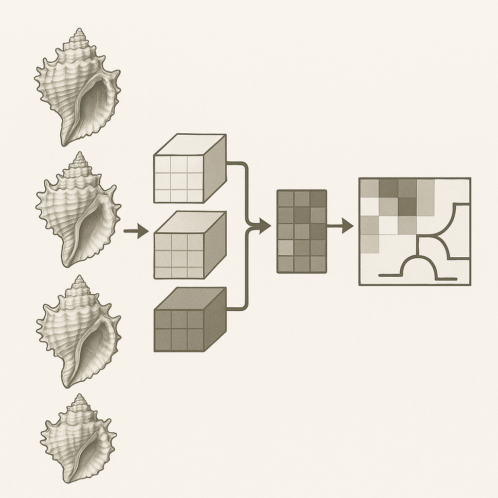
Feature vectors from the the penultimate layer of the trained Oxymeris CNN model
To analyze the internal representations learned by the Oxymeris CNN model, we extracted high-dimensional feature vectors from the penultimate layer of the trained network.
These embeddings capture rich semantic information about each image while abstracting away from pixel-level details. The model was implemented and trained using TensorFlow,
and feature vectors were obtained using Keras’ Model subclassing, where a truncated version of the network outputs activations from the final convolutional or dense layer
prior to classification. Each image in the dataset was passed through the network in inference mode, and the resulting feature vector (1408 dimensions) was stored for
further analysis.
To quantify similarity between images, we computed pairwise cosine similarity between feature vectors.
For each image , compute similarity to all other images in the same class:
and are the feature vectors (or embeddings) corresponding to image and image , respectively. These are extracted from the penultimate layer of the trained CNN and represent the model's internal encoding of visual characteristics in a high-dimensional space.
Cosine similarity measures the cosine of the angle between two vectors in the embedding space, and is particularly well-suited for high-dimensional data where the magnitude of the vectors is less informative than their direction. It was calculated using the sklearn.metrics.pairwise.cosine_similarity function from scikit-learn. Cosine distance (1 - similarity) was used when required for clustering, outlier detection, or visualization purposes. This approach allowed us to evaluate both intra-class cohesion and inter-class separation based on the learned feature representations, providing a model-centric view of image similarity beyond what can be captured by raw pixel comparisons.
CNN NJ analysis
The CNN-based morphological tree was constructed by aggregating deep visual features extracted from a trained convolutional neural network model. First, species-level representations were obtained by averaging the feature vectors of individual images per species, resulting in a feature matrix of shape (13 species × F features). To account for variation and assess cluster robustness, we applied a non-parametric bootstrapping strategy: for each of 500 replicates, the feature dimensions (columns) were resampled with replacement, and cosine distances were computed between species. These distance matrices were converted into phylogenetic distance matrices and used to infer neighbor-joining (NJ) trees via the DendroPy library.
Across all replicates, bipartitions (internal nodes) were encoded and tallied to compute their frequency of occurrence. For each unique bipartition present in ≥50% of replicates, a majority-rule consensus tree was constructed. Branch lengths were set to the mean length observed for each split across replicates, and bootstrap support values were annotated as the percentage of trees in which each bipartition appeared. To ensure consistency with the molecular dataset, either all 13 species or a subset of 8 species overlapping with the sequence-based tree were included, depending on the analysis. The resulting consensus trees were exported in Newick format and visualized using ETE3, with species labels, support values, and branch lengths graphically rendered for interpretability.
Comparing morphological trees
To evaluate the impact of tree construction method on species relationships inferred from morphological features, we compared a Neighbor-Joining (NJ) tree with a hierarchical clustering tree constructed using the average linkage (UPGMA) algorithm. Both trees were derived from the same CNN-based morphological distance matrix computed from species-level averaged feature vectors. The NJ tree was inferred using the nj() function from the scikit-bio library, while the UPGMA tree was generated via the scipy.cluster.hierarchy.linkage() function with the 'average' method applied to a condensed distance matrix. To assess topological differences, we computed the Robinson–Foulds (RF) distance using ete3, which quantifies the number of bipartitions that differ between two unrooted trees. This metric provides an objective measure of topological similarity between the trees, independent of branch lengths.
Oxymeris phylogenetic trees
To extract the phylogenetic relationships among species of the genus Oxymeris, we pruned the full Terebridae species tree to retain only terminal taxa of the genus Oxymeris. The tree was previously inferred from concatenated DNA sequence alignments using a species tree approach, and encoded in extended Newick format with metadata annotations. The pruning and visualization were conducted using the ete3 toolkit in Python. Branch lengths were preserved from the original tree, and internal support values were extracted from the pp1 metadata tag embedded in node labels. These posterior probabilities represent support from gene-tree reconciliation and were annotated below each internal node in the resulting subtree.
Comparing morphological and molecular tree
To quantify topological similarity between the morphology-based and molecular phylogenies, we again computed the Robinson–Foulds (RF) distance using the ete3 library in Python. Prior to comparison, we ensured that both trees contained identical sets of taxa by pruning and standardizing leaf names. The RF distance was computed in unrooted mode, and normalized by the maximum possible RF distance given the shared set of taxa (see also 'Comparing morphological trees'). This normalization yields a tree similarity score between 0 (completely different) and 1 (identical).
To assess the correspondence between the molecular and CNN-derived morphological distance matrices, we performed a Mantel test using the skbio Python package. The test evaluates the correlation between two symmetric distance matrices of equal dimensions using Pearson’s correlation coefficient, with 999 permutations to assess statistical significance. The molecular distance matrix was derived from distances on the phylogeny inferred from sequence data, while the morphological matrix was based on pairwise cosine distances computed from species-level CNN feature vectors. Both matrices were aligned to ensure the same taxon ordering, symmetrized to enforce strict matrix symmetry, and formatted as required by the Mantel test.
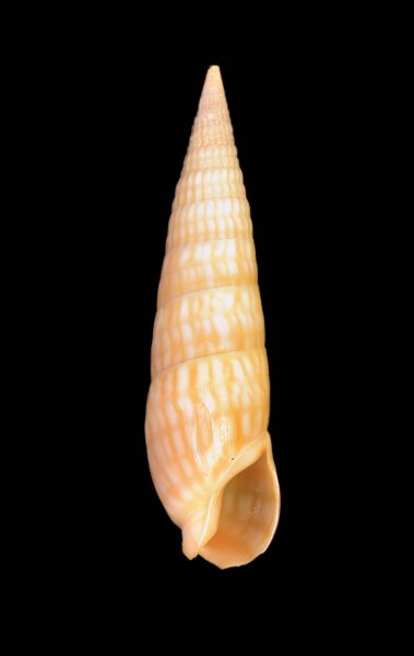
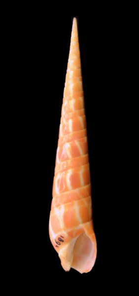
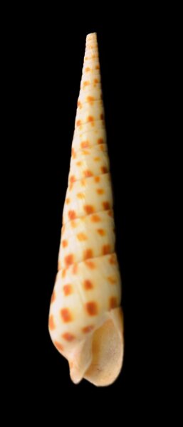
Figure 1: Representative images of Oxymeris species used in this study. Examples of shell images from the dataset, illustrating the morphological diversity within the genus Oxymeris. The CNN was trained to distinguish species based on visual features such as shell shape, color patterns, and ornamentation. From left to right: Oxymeris cerithina, O. dimidiata, and O. areolata.
Results
CNN model
The CNN model trained for Oxymeris species identification achieved strong classification performance, as reflected in both overall metrics and per-species results. The final training accuracy reached 98%, with a validation accuracy of 95%, indicating good generalization to unseen data. Although some degree of overfitting is evident — given that validation accuracy is slightly lower than training accuracy — the corresponding loss values (training loss: 0.093, validation loss: 0.224) remain well within acceptable ranges, suggesting stable training dynamics and effective convergence.
A detailed breakdown of performance by species is provided in Table II, which lists recall, precision, and F1-score for each of the 13 Oxymeris species. These metrics reveal high classification fidelity across most taxa, with eight species achieving an F1-score of 0.95 or higher. Notably, Oxymeris areolata, O. dimidiata, and O. trochlea attained perfect scores across all metrics, reflecting unambiguous species-level discrimination by the model. The more challenging species — such as O. maculata and O. crenulata — still achieved F1-scores above 0.89 and 0.91 respectively, indicating reliable, albeit slightly lower, classification accuracy.
Table II. Species-level classification performance of the CNN model
| Species | # images | Recall | Precision | F1 |
|---|---|---|---|---|
| Oxymeris areolata (Link, 1807) | 339 | 1.000 | 1.000 | 1.000 |
| Oxymeris cerithina (Lamarck, 1822) | 221 | 1.000 | 0.973 | 0.986 |
| Oxymeris chlorata (Lamarck, 1822) | 163 | 0.946 | 0.946 | 0.946 |
| Oxymeris crenulata (Linneaus, 1758) | 396 | 0.905 | 0.927 | 0.916 |
| Oxymeris dillwynii (Deshayes, 1857) | 67 | 0.909 | 0.833 | 0.870 |
| Oxymeris dimidiata (Linneaus, 1758) | 263 | 1.000 | 1.000 | 1.000 |
| Oxymeris fatua (Hinds, 1844) | 66 | 1.000 | 0.923 | 0.960 |
| Oxymeris felina (Dillwyn, 1817) | 155 | 0.966 | 0.933 | 0.949 |
| Oxymeris gouldi (Deshayes, 1857) | 56 | 0.938 | 1.000 | 0.968 |
| Oxymeris maculata (Linneaus, 1758) | 237 | 0.875 | 0.913 | 0.894 |
| Oxymeris senegalensis (Lamarck, 1822) | 186 | 1.000 | 0.974 | 0.987 |
| Oxymeris strigata (G. B. Sowerby I, 1825) | 46 | 0.875 | 1.000 | 0.933 |
| Oxymeris trochlea (Deshayes, 1857) | 61 | 1.000 | 1.000 | 1.000 |
| This table provides a detailed breakdown of the model's classification performance for each of the 13 Oxymeris species included in the study. # images indicates the total number of images used for each species. Recall (Sensitivity) measures the model's ability to correctly identify all images of a given species. Precision measures the proportion of correct identifications among all images assigned to a species. The F1-score is the harmonic mean of precision and recall, providing a single metric for overall accuracy per species. Values approaching 1.0 indicate high performance. | ||||
In aggregate, the macro-averaged performance (which treats all species equally) yielded a recall of 0.955, precision of 0.956, and F1-score of 0.954, confirming balanced performance across classes regardless of image count. The weighted averages, which account for the differing number of images per species, were slightly higher: recall and precision at 0.957–0.958, and F1-score at 0.957. These figures highlight the model’s robustness, showing it performs well both on common and rarer species. Overall, the CNN effectively captures interspecific morphological variation, enabling accurate, image-based identification of Oxymeris species at scale.
Table III. Pairwise cosine similarity matrix of Oxymeris species based on CNN feature vectors.
| Species | areolata | cerithina | chlorata | crenulata | dillwynii | dimidiata | fatua | felina | gouldi | maculata | senegalensis | strigata | trochlea |
|---|---|---|---|---|---|---|---|---|---|---|---|---|---|
| areolata | 1.00 | ||||||||||||
| cerithina | 0.31 | 1.00 | |||||||||||
| chlorata | 0.62 | 0.69 | 1.00 | ||||||||||
| crenulata | 0.55 | 0.66 | 0.76 | 1.00 | |||||||||
| dillwynii | 0.36 | 0.77 | 0.68 | 0.77 | 1.00 | ||||||||
| dimidiata | 0.50 | 0.60 | 0.63 | 0.56 | 0.60 | 1.00 | |||||||
| fatua | 0.33 | 0.77 | 0.61 | 0.67 | 0.82 | 0.69 | 1.00 | ||||||
| felina | 0.61 | 0.55 | 0.76 | 0.76 | 0.67 | 0.55 | 0.67 | 1.00 | |||||
| gouldi | 0.28 | 0.78 | 0.60 | 0.72 | 0.79 | 0.60 | 0.75 | 0.53 | 1.00 | ||||
| maculata | 0.53 | 0.59 | 0.79 | 0.81 | 0.60 | 0.43 | 0.59 | 0.68 | 0.57 | 1.00 | |||
| senegalensis | 0.54 | 0.70 | 0.76 | 0.74 | 0.77 | 0.59 | 0.66 | 0.55 | 0.78 | 0.71 | 1.00 | ||
| strigata | 0.60 | 0.62 | 0.67 | 0.65 | 0.66 | 0.58 | 0.61 | 0.60 | 0.56 | 0.57 | 0.73 | 1.00 | |
| trochlea | 0.30 | 0.63 | 0.50 | 0.66 | 0.65 | 0.70 | 0.63 | 0.46 | 0.82 | 0.41 | 0.60 | 0.50 | 1.00 |
| This matrix quantifies the morphological similarity between species as learned by the CNN. Each cell contains the cosine similarity value between the averaged feature vectors of two species. Values range from 0 to 1, where 1 (along the diagonal) represents perfect self-similarity. Higher off-diagonal values (e.g., > 0.80) indicate that the model perceives two species as very similar in shell morphology, while lower values (e.g., < 0.40) indicate high distinctiveness in the learned feature space. | |||||||||||||
The table III matrix reveals varying degrees of inter-species similarity. Notably, some species pairs, such as O. gouldi and O. trochlea, as well as O. crenulata and O. maculata, exhibit high cosine similarity (≥ 0.80), suggesting that their feature representations are closely aligned, which could explain potential confusion during classification. In contrast, species like O. areolata versus O. gouldi or O. trochlea display low similarity (≤ 0.3), indicating that the model has learned distinct feature representations for these classes. These insights complement traditional confusion matrix analysis by offering a feature-space-level perspective on class separability.
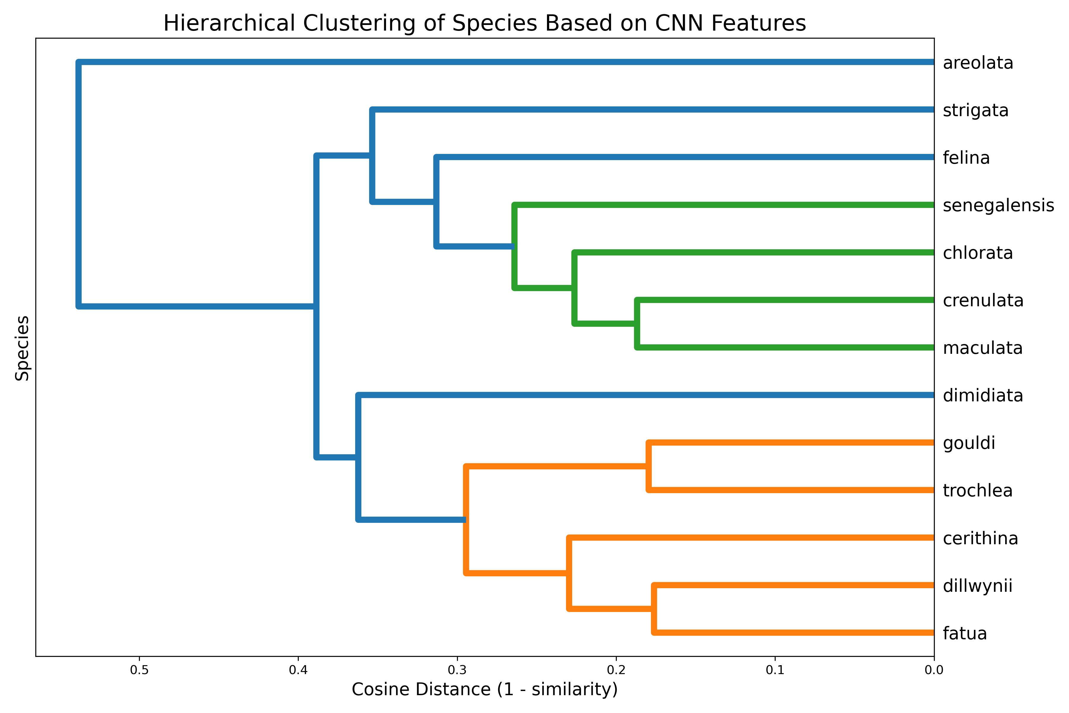
Figure 2:Hierarchical clustering of Oxymeris species based on CNN-derived morphological distances. This dendrogram illustrates the phenetic relationships among the 13 Oxymeris species based on their visual similarity. The tree was constructed using the Unweighted Pair Group Method with Arithmetic Mean (UPGMA) algorithm applied to a matrix of pairwise cosine distances (calculated as 1 - cosine similarity) between the species-averaged feature vectors. Species that cluster together with shorter branch heights are interpreted by the CNN as being more morphologically similar.
The dendrogram (figure 2) presents a hierarchical clustering of species based on cosine distance (1 – similarity) between their class centroids. Species that are closer in the CNN’s feature space are grouped together at lower linkage distances. The tree structure highlights clusters of visually or morphologically similar species. For instance, the close clustering of O. dillwynii, O. fatua, and B. cerithina suggests these classes are tightly related in the model’s internal representation. The hierarchical structure helps identify broader groupings and potential taxonomy - like relationships learned by the CNN, even in the absence of explicit hierarchical labels.

Figure 3: Neighbor-joining consensus tree of Oxymeris species based on CNN morphological features. Phylogenetic hypothesis for Oxymeris based solely on CNN-derived morphological data. This is a 50% majority-rule consensus tree from 500 bootstrap replicates. The tree was inferred using the neighbor-joining (NJ) algorithm from the cosine distance matrix. Numbers at the nodes represent bootstrap support percentages, indicating the frequency at which a given clade appeared in the replicates. Branch lengths are proportional to the mean cosine distance between nodes.
The image-based tree inferred from CNN-derived morphological features of 13 Oxymeris species reveals several well-supported clades and structured patterns of similarity. The consensus tree, constructed from 500 bootstrap replicates using cosine distances between species-level feature vectors, includes bootstrap support values and averaged branch lengths, highlighting the robustness and relative distinctiveness of certain species groupings.
Two major clades emerge from the tree. The upper clade includes O. strigata, O. senegalensis, and O. dimidiata, alongside a highly supported subclade uniting O. gouldi and O. trochlea (100% bootstrap), which is itself sister to O. cerithina, O. dillwynii, and O. fatua. Bootstrap support for these nodes ranges from 73% to 100%, indicating moderate to high stability in the groupings. The lower clade includes O. chlorata, O. crenulata, O. maculata, and O. areolata, with O. felina forming a distinct, early-branching lineage. Notably, O. crenulata and O. maculata cluster together with 77% support, while O. chlorata forms a separate lineage with weak support (3%), possibly reflecting ambiguity in its morphological placement.
Branch lengths vary across the tree, with relatively long branches observed for O. areolata (0.272), O. dimidiata (0.206), and O. strigata (0.145), suggesting higher morphological distinctiveness in CNN feature space. In contrast, closely related taxa such as O. gouldi and O. trochlea or O. dillwynii and O. fatua exhibit short internodes, indicating greater similarity. Overall, the tree structure suggests that CNN-extracted visual features capture meaningful interspecific differences, with several clusters aligning with intuitive morphological expectations and displaying high bootstrap support.
The comparison between the UPGMA and NJ trees revealed a Robinson–Foulds distance of 10 out of 20, yielding a normalized RF distance of 0.500 and a tree similarity score of 0.500. This indicates that exactly half of the internal branches (bipartitions) are shared between the two trees, reflecting a moderate level of topological congruence. This result is consistent with theoretical expectations, given that the NJ algorithm seeks to globally optimize tree additivity without assuming equal rates of divergence, whereas UPGMA enforces an ultrametric structure and merges taxa based on local similarity. The observed divergence between the trees may also reflect non-additive structure in the morphological distance space or feature interactions not fully captured by hierarchical linkage rules. Overall, this comparison shows that while CNN-derived morphological distances do carry phylogenetic signal, the method of tree reconstruction can substantially influence the inferred relationships among species.

Figure 4: Tanglegram comparing the topologies of the NJ and UPGMA morphological trees.
A visual comparison of the tree topologies generated by two different algorithms from the same morphological distance matrix. The neighbor-joining (NJ) tree is on the left,
and the hierarchical clustering (UPGMA) tree is on the right. Lines connect the same species across both trees. Crossing lines indicate topological incongruence.
The normalized Robinson–Foulds (RF) distance between these two trees is 0.5, meaning they share only half of their bipartitions. This highlights how the choice
of tree-building algorithm can influence inferred relationships from the same dataset.
A tanglegram visualization (Figure 4) illustrates the relative placement of species in the CNN-based Neighbor-Joining (left) and Hierarchical Clustering (right) trees. While several species (e.g., O. areolata, O. fatua) maintain consistent positions, others (e.g., O. gouldi, O. dimidiata, O. chlorata) show divergent placements. However, as emphasized by de Vienne (2019), such visualizations are sensitive to leaf ordering and layout, and crossing lines should not be directly interpreted as a quantitative measure of topological incongruence. We therefore rely on formal metrics such as the Robinson–Foulds distance (0.5) to assess tree similarity.
Comparison of species groupings across the CNN-based Neighbor-Joining and complete-linkage trees revealed both stable and unstable clades. Species like O. strigata and O. senegalensis consistently grouped together, indicating robust morphological similarity across methods. In contrast, species such as O. areolata, O. felina, and O. chlorata shifted groupings depending on the clustering strategy, suggesting intermediate or ambiguous morphological traits in CNN feature space. These topological shifts may reflect morphological convergence, high intraspecific variability, or limitations in how the CNN encodes relevant shell features.
The use of UPGMA (average linkage) and Neighbor-Joining (NJ) reflects different inferential goals: UPGMA clusters taxa based on overall morphological similarity and assumes constant evolutionary rates, whereas NJ seeks to reconstruct divergence patterns without enforcing ultrametric constraints. Given these foundational differences, the moderate topological disagreement observed between the UPGMA and NJ trees is not only expected but informative — it reveals to what extent morphological similarity, as captured by CNN features, mirrors the structure of evolutionary divergence.
The methodological comparison demonstrated that while UPGMA provides insight into overall visual similarity, it diverges from the NJ tree when applied to the same morphological distance data (normalized RF distance ≈ 0.5). Given that UPGMA assumes ultrametricity — a condition unlikely met in CNN-derived feature space — the NJ method is more appropriate for phylogenetic interpretation. Thus, following consensus in the phylogenetics community [arXiv, Wikipedia], we proceeded with the NJ-derived tree for all downstream evolutionary comparisons with the molecular phylogeny. This approach ensures that inferred relationships reflect divergence patterns rather than phenotype similarity artifacts.
Oxymeris Phylogenetic tree

The pruned Oxymeris subtree comprises 11 species and retains both branch lengths and internal support values from the full Oxymeris phylogeny (Fig. 5). The topology reveals two well-supported clades: one comprising O. consors, O. dimidiata, O. areolata, and O. crenulata, with internal nodes supported by posterior probabilities up to 0.94; and a second cluster grouping O. caledonica, O. felina, O. cerithina, and O. strigata, although with lower average support (ranging from 0.40 to 0.67). The sister-group relationship between O. chlorata and O. maculata is also moderately supported (pp1 = 0.78), and both are separated from the rest of the Oxymeris by relatively long branches. The topology provides a reference framework for comparing morphological signal extracted from CNN-based image embeddings against molecular phylogenetic relationships.

Figure 6: Pruned molecular phylogeny of Oxymeris showing species shared with the morphological analysis. The evolutionary reference tree used for direct comparison with the morphological data. This tree is a subtree of the full molecular phylogeny (shown in Fig. 5) and has been pruned to retain only the eight species that are also present in the morphological analysis (Fig. 7). Numbers at the nodes represent posterior probability support values. Branch lengths are proportional to the number of substitutions per site.

Figure 7: Pruned morphological neighbor-joining tree of Oxymeris and its comparison to the molecular phylogeny. The phenetic relationships among the eight common Oxymeris species as inferred from CNN features. This tree is a subtree of the full morphological tree (shown in Fig. 3) and was inferred using the neighbor-joining (NJ) algorithm from a cosine distance matrix. Numbers at the nodes are bootstrap support percentages.
Comparison of the morphological and molecular tree
The CNN-derived morphology tree and the molecular phylogeny shared 8 terminal taxa. The Robinson–Foulds (RF) distance between both trees was 10 out of 10, resulting in a normalized RF distance of 1.000 and a tree similarity score of 0.000. This indicates that the two trees do not share any internal bipartitions, and are therefore topologically incongruent. The result further supports the conclusion that the CNN feature representations capture limited phylogenetic signal relative to the molecular data.
The Mantel test revealed no significant correlation between the molecular and CNN-based morphological distance matrices (Mantel r = 0.006, p = 0.966). This lack of association suggests that the pairwise similarities captured by CNN features do not align with the evolutionary distances inferred from genetic data. Together with the Robinson–Foulds result, this further supports the interpretation that morphological similarity extracted by CNNs captures patterns distinct from phylogenetic divergence, potentially reflecting ecological convergence, phenotypic plasticity, or visual homoplasy.
Discussion
The CNN model achieved excellent accuracy across most Oxymeris species, with macro‑ and weighted‑average F1 scores around 0.95 and individual species such as O. areolata and O. dimidiata classified perfectly. These high scores confirm that deep learning can extract discriminative visual features from shell images, providing a practical tool for rapid species identification. The cosine‑similarity matrix revealed both tight and diffuse clusters in feature space: species pairs like O. gouldi–O. trochlea and O. crenulata–O. maculata showed high similarity (≥ 0.80), whereas O. areolata versus O. gouldi or O. trochlea had low similarity (≤ 0.3), indicating that the network has learned class‑specific features. Such feature‑space insights complement the confusion matrix and pinpoint species where morphological overlap could cause misclassification. Nevertheless, some taxa with moderate similarity (e.g. O. felina, O. chlorata) still achieved high F1 scores, suggesting that the network can capture subtle patterns beyond overall cosine similarity.
Despite strong classification performance, our analyses show that CNN‑derived morphological distances do not reflect evolutionary divergence. The Mantel test between the CNN‑based cosine‑distance matrix and the molecular distances was essentially zero (r = 0.006, p = 0.966), and the Robinson–Foulds comparison between the molecular and morphological trees found no shared internal bipartitions. These results align with earlier warnings that shell morphology in Terebridae can be deceptive: Puillandre and Holford (2010) [1] reported that many shell characters used to define genera correspond to convergent or ancestral polymorphisms, causing specimens assigned to “Terebra” to fall into three distinct molecular clades [1]. They argued that species definitions based solely on shells are prone to error and that shell variation can result from environmental variability rather than shared ancestry [1]. In our dataset, species such as O. chlorata and O. felina occupy inconsistent positions across trees, suggesting that CNN features capture superficial morphology influenced by factors like coloration, ribbing patterns or size, which may not track phylogeny. The absence of correlation underscores that image‑based phenetic similarity and evolutionary distance are decoupled in auger snails, likely due to widespread morphological convergence, phenotypic plasticity and ecological adaptation.
Our comparison of tree‑building methods further illustrates how algorithmic assumptions shape inferred relationships. When the same distance matrix was input, the UPGMA tree shared only half of its bipartitions with the NJ tree (normalized RF = 0.5). This moderate incongruence is expected because UPGMA assumes a strict molecular clock and clusters taxa based on overall similarity, whereas NJ optimizes tree additivity without imposing ultrametric constraints. The NJ method is generally preferred for phylogenetic inference when distances are not clock‑like, which is almost certainly the case for CNN features. Within the NJ consensus tree, we observed two well‑supported clades: an upper group containing O. strigata, O. senegalensis, O. dimidiata and a subclade of O. gouldi + O. trochlea; and a lower group containing O. chlorata, O. crenulata, O. maculata, O. areolata with O. felina as an early branch. However, the placement of some taxa — especially O. chlorata and O. felina—showed low support or long branches, hinting at ambiguous morphology. These morphological clades have no counterparts in the molecular tree, which emphasises that CNN features may group species by shell colour or ornamentation rather than shared ancestry.
Several factors could contribute to the weak phylogenetic signal in CNN features. Sampling limitations are a major concern: nine Oxymeris species were excluded due to insufficient imagery, and some included taxa had relatively few images. Uneven sample sizes can bias feature averaging and distance estimation, while misidentifications in online image repositories could introduce noise. Photographs varied in lighting, orientation and background despite preprocessing; such variability may cause CNNs to learn non‑biological artefacts like shadows or camera angles. Moreover, the network was trained to maximise classification accuracy rather than preserve phylogenetic relationships. It likely emphasises conspicuous traits—colour patterns, rib spacing or shell spire proportions — that may evolve rapidly under ecological selection or phenotypic plasticity. Puillandre and Holford note that the molluscan shell is highly plastic, and morphological variation may reflect environmental conditions [1]. Consequently, even perfectly identified shells may exhibit divergent CNN features if collected from different habitats or growth stages.
Looking ahead, improvements in data quality and modelling could enhance the phylogenetic utility of image embeddings. Expanding the dataset to include all Oxymeris species with balanced image counts and standardised photographic conditions would reduce noise and sampling bias. Incorporating side and aperture views could capture shape features that are more evolutionarily conserved. Feature extraction could be refined using geometric morphometric landmarks or self‑supervised learning that prioritises structural traits over texture and colour. Integrating ecological metadata (e.g., locality, habitat) might help disentangle environmentally induced variation from inherited morphology. Importantly, machine‑vision representations should be combined with traditional morphological characters and molecular data in a total‑evidence framework. Such integrative analyses would allow CNN‑derived features to contribute to species delimitation while safeguarding against misleading signal.
From a taxonomic and conservation standpoint, our results highlight both the promise and limitations of deep learning for malacology. CNNs provide rapid, scalable identification tools that can aid biodiversity surveys, fisheries management and citizen science. However, they should not be used in isolation to infer phylogenetic relationships or synonymise taxa. Our findings support calls by Modica et al. (2020) [4] and Fedosov et al. (2020) [5] to base terebrid classifications on DNA diagnoses coupled to detailed morphological descriptions Shell images and CNN embeddings can still flag candidate cryptic species, reveal patterns of morphological convergence or divergence, and enrich phenotypic datasets for evolutionary studies. Ultimately, a multi‑modal approach that leverages genetics, anatomy and machine vision offers the most robust path forward for resolving auger snail diversity and understanding the selective pressures shaping their remarkable shells.
References
- [1] Puillandre N, Holford M. The Terebridae and teretoxins: Combining phylogeny and anatomy for concerted discovery of bioactive compounds. BMC Chem Biol. 2010 Sep 17;10:7 (2010)
- [2] Eiseul K et al. Deep learning-based phenotype classification of three ark shells: Anadara kagoshimensis, Tegillarca granosa, and Anadara broughtonii. Frontiers in Marine Science, Volume 11 (2024)
- [3] Ph. Kerremans Technical Reports for a Total-Evidence Phylogenetics of Terebridae. Identifyshell.org (2025)
- [4] Modica, M. V., Gorson, J., Fedosov, A. E., et al. Macroevolutionary analyses suggest that environmental factors, not venom apparatus, play key role in Terebridae marine snail diversification. Systematic Biology 69 (3): 413–430 (2020)
- [5] Fedosov, A. E., Malcolm, G., Terryn, Y., et al. Phylogenetic classification of the family Terebridae (Neogastropoda: Conoidea). Journal of Molluscan Studies 86: 1–29 (2020)
- [6] M Holford et al. Evolution of the Toxoglossa Venom Apparatus as Inferred by Molecular Phylogeny of the Terebridae. Mol. Biol. Evol. 26(1):15–25. (2009)
- [7] Powers, D. M. W. Evaluation: From Precision, Recall and F-measure to ROC, Informedness, Markedness & Correlation. Journal of Machine Learning Technologies, 2(1), 37–63. (2011)
- [8] Zhang, Q., Zhou, J., He, J. et al. A shell dataset, for shell features extraction and recognition.. Nature, Sci Data 6, 226 (2019)