Fine-tuning EfficientNetV2 Models
Published on: 21 December 2024
Abstract
EfficientNetV2, a family of convolutional neural networks, has gained significant attention in computer vision due to its impressive speed and parameter efficiency. While these models are pre-trained on large datasets like ImageNet, fine-tuning them on specific tasks and datasets can further enhance their performance. EfficientNetV2 is a new family of convolutional networks that builds upon the success of its predecessor, EfficientNet, by addressing its training bottlenecks and introducing architectural improvements. EfficientNetV2 models train much faster than state-of-the-art models while being up to 6.8x smaller [1, 3]. Experimenting with different hyperparameters have shown that fine-tuning increases accuracy often with more than 5%. The optimal number of top layers to unfreeze during training is around 60 for EfficientNetV2B2. To prevent overfitting a strong regularization is needed.
Introduction
EfficientNetV2 models achieve faster training speed and better parameter efficiency than previous models. This is achieved through a combination of
training-aware neural architecture search and scaling, which jointly optimize training speed and parameter efficiency . EfficientNetV2 models can be trained
efficiently at a large scale. They outperform Vision Transformers in terms of both accuracy and training efficiency. For example, by pretraining on the same
ImageNet21k, EfficientNetV2 achieves 87.3% top-1 accuracy on ImageNet ILSVRC2012, outperforming the recent ViT by 2.0% accuracy while training 5x-11x faster
using the same computing resources [1].
The development of EfficientNetV2 was motivated by addressing the training bottlenecks of EfficientNetV1.
For example, training EfficientNetV1 with very large image sizes was slow, and depthwise convolutions in the early layers were also slow .
Another study explored the impact of scaling up datasets on model accuracy . The researchers found that scaling up the dataset, rather than simply
increasing the model size, is more effective for achieving high accuracy (above 85%). They also implemented techniques like reducing training epochs
to 60 or 30, using cosine learning rate decay, and normalizing labels to sum to 1 before computing softmax loss to improve performance [1,
4].
Fine-tuning an EfficientNetV2 model involves adjusting its weights to improve performance on a specific task and dataset. An approach is to start by freezing the initial layers of the model to retain the learned features from the pre-trained model. These early layers often capture generic features that are useful across different tasks. As training progresses, gradually unfreeze layers to allow for fine-tuning of higher-level features, which are more specific to the target task [2].
Methods
We used the Harpa genus dataset for these tests. It is an average size dataset of 5837 images, with 13 species. All runs were done with EfficientNet V2 B2 [1], which uses ImageNet for transfer learning. Several hyperparameters were kept constant during model creation:
Fixed hyperparameters
| Hyperparameter | Value | Comments |
|---|---|---|
| Batch Size | 64 | The batch size determines the number of samples processed in each iteration. It affects training speed and memory usage. We assume this parameter is not influencing fine-tuning results. |
| Epochs | 50 | The number of epochs determines how many times the entire training dataset is passed through the model. Because early-stopping is used, often less than 50 epochs were needed. Fine-tuning usually requires fewer epochs compared to training from scratch. |
| Optimizer | Adam | The optimizer determines the algorithm used to update model weights during training. |
Results
Learning rate.
The learning rate is an important parameter during fine-tuning. Keeping all other parameters fixed, a learning rate between 0.5 and 0,00005 was tested. For the results shown in the table below, the 30 top layers were made trainable. A regulation value of 0.0001 was used.| Learning rate | 0.5 | 0.05 | 0.005 | 0.001 | 0.0005 | 0.0001 | 0.00005 |
| Validation Accuracy | 0.877 | 0.91 | 0.921, 0.933 | 0.934, 0.942 | 0.927 | 0.919 | 0.913 |
Impact of unfreezing the number of top layers.
EfficientV2B2 is a complex model, having more than 300 layers. We have tested unfreezing a wide range of top layers (or made top layers trainable).| # unfreezed layers | 0 | 3 | 6 | 15 | 30 | 60 | 90 | 120 | 150 | 180 |
| Validation Accuracy | 0.879 | 0.907 | 0.898 | 0.901, 0.925 | 0.934, 0.942 | 0.938, 0.933 | 0.933 | 0.929 | 0.946 | 0.938 |
Regularization to prevent overfitting.
To prevent overfitting when unfreezing top layers, runs we various values of dropout of the top layer and regularization were tested.| Run 1 | Run 2 | Run 3 | Run 4 | Run 5 | Run 6 | |
|---|---|---|---|---|---|---|
| regularization | 0.0001 | 0.005 | 0.1 | 0.005 | 0.01 | 0.1 |
| dropout | 0.2 | 0.2 | 0.5 | 0.2 | 0.5 | 0.5 |
| #unfreezed layers | 30 | 30 | 30 | 60 | 60 | 60 |
| Training Accuracy | 0.949 | 0.978 | 0.979 | 0.982 | 0.976 | 0.991 |
| Validation Accuracy | 0.921 | 0.940 | 0.943 | 0.938 | 0.936 | 0.946 |
| Training Loss | 0.244 | 0.145 | 0.364 | 0.098 | 0.313 | 0.216 |
| Validation Loss | 0.287 | 0.266 | 0.399 | 0.293 | 0.443 | 0.334 |
Discussion
Utilizing ImageNet for initial transfer learning typically provides a model with a significant performance boost, owing to the extensive and varied nature
of the dataset. ImageNet's rich feature set, developed from a broad spectrum of image classes, furnishes the model with a robust foundation of generalizable
visual features. This pre-training often results in substantial improvements in model accuracy, even before any domain-specific fine-tuning is undertaken.
However, achieving further refinements in performance—specifically, improvements beyond 5% - necessitate extensive fine-tuning of many layers within the model.
This requirement becomes particularly critical when the target domain encompasses image classes or features markedly absent from ImageNet. For instance,
ImageNet does not include classes for mollusc shells, a category with distinct textural and morphological characteristics not typically encountered in the dataset.
When the target domain diverges significantly from ImageNet's scope, as with mollusc shells, the generic lower and mid-level features pre-trained on ImageNet
might not align well with the specialized needs of the new domain. These foundational features, essential for initial pattern recognition and texture analysis,
may be inadequate for capturing the unique aspects of such specialized images.
In such scenarios, fine-tuning a broader array of layers becomes helpful. By adjusting deeper layers of the network, the model can re-learn and adapt these
fundamental features to better suit the specific requirements of the new domain. This extensive fine-tuning allows the model to overhaul its basic feature
detectors and classifiers, making them more sensitive to the unique attributes of the target images. Such a deep and comprehensive modification not only
enhances the model’s accuracy on the new domain but also broadens its ability to generalize from more nuanced and domain-specific visual data.
Moreover, this approach underscores the adaptive capacity of neural networks through transfer learning, highlighting how even well-established pre-trained
models like those trained on ImageNet can be recalibrated to tackle substantially different visual tasks effectively.
When making a substantial number of layers trainable, there is a increased risk of overfitting, as the model gains the capacity to finely tune itself
to the idiosyncrasies of the training data rather than learning to generalize to unseen data. To mitigate this risk, it is crucial to employ robust
strategies such as increasing dropout rates and applying more rigorous regularization techniques.
Incorporating higher dropout values helps by randomly deactivating a portion of the neurons in the unfrozen layers during training,
which prevents the network from becoming overly dependent on any single or small group of features. This encourages the model to develop a more
distributed and robust internal representation, enhancing its generalization capabilities.
Similarly, intensifying the regularization — by raising the coefficients in regularization — penalizes the model for overly complex
configurations that fit too closely to the noise in the training data. This not only helps in reducing overfitting but also ensures that the model's
adaptations are meaningful and contribute positively to its ability to perform well on new, unseen data.
The careful calibration of dropout and regularization levels, therefore, plays a pivotal role. This strategy ensures that the model
retains a significant capacity for learning and adapting to new data, without compromising its ability to generalize.
Such a balanced approach is crucial for maintaining the delicate equilibrium between fitting the training data well and performing effectively
on validation or test data, thus ensuring the model is both powerful and practical for identifying molluscs.
References
- [1] Mingxing Tan and Quoc V. Le EfficientNetV2: Smaller Models and Faster Training. Proceedings of the 38th International Conference on Machine Learning, 2021.
- [2] restack Fine-Tuning EfficientNet Techniques. restack, 2024.
- [3] Yixing Fu Image classification via fine-tuning with EfficientNet. Keras.io, 2020.
- [4] Ritvik Rastogi Papers Explained 233: EfficientNetV2. Medium, 2024.
