Technical Report: Phylogenetic Analysis of the ribosomal DNA genes: 12s, 16s, 28s
Published on: July 2025
Abstract
A phylogenetic analysis of the Terebridae based on all publicly available rDNA markers (mitochondrial 12S rRNA, 16S rRNA; nuclear 28S rRNA). We retrieved 1 346 sequences from NCBI, validated taxonomic identifications via MolluscaBase/WoRMS, and generated concatenated alignments using MAFFT. Maximum‑likelihood and Bayesian trees were inferred in IQ‑TREE and BEAST, respectively, with topology imbalance assessed via normalized Colless’ and Sackin indices against 200 coalescent simulations. The BEAST maximum‑clade‑credibility tree, selected as our molecular “backbone,” exhibits diversification patterns consistent with a birth–death process under incomplete sampling. This reference phylogeny will serve to benchmark convolutional neural networks trained on shell imagery, enabling an evaluation of morphological versus molecular signals in gastropod evolution.
Introduction
Ribosomal DNA (rDNA) markers — namely the mitochondrial 12S and 16S small-subunit genes and the nuclear 28S large-subunit gene — have proven invaluable for reconstructing both deep and shallow divergences in molluscan lineages. The slower-evolving 28S region provides resolution among major clades, while the more variable mitochondrial ribosomal genes clarify relationships among congeners. Previous studies (e.g., Holford et al., 2009 [5]; Modica et al., 2020 [6]) have utilized these loci, but no analysis has yet integrated all sequences from all publications of public Terebridae sequences.
In this study, we mined the National Center for Biotechnology Information (NCBI) database for all available Terebridae rDNA sequences, cross-validated taxonomic identifications against MolluscaBase/WoRMS, and assembled a data set comprising 12S, 16S, and 28S loci. We then infer a baseline phylogenetic tree from concatenated Cox1 (previous report) 12S, 16S, and 28S alignments.
Our primary objective is to establish this molecular backbone tree as a reference against which to compare phylogenies generated by convolutional neural network (CNN) models trained on shell images. By evaluating whether CNN-derived feature spaces recapitulate rDNA-based relationships, we aim to test whether visual shell characters carry a phylogenetic signal detectable by deep-learning approaches. This combined molecular–computational framework will not only benchmark CNN performance in systematic inference but also explore the potential of image-based models to uncover evolutionary patterns in gastropod morphology.
Methods
Data Collection
All sequences were retrieved from https://www.ncbi.nlm.nih.gov/gene/ using search expression "Terebridae"[Organism] OR Terebridae[All Fields]. A total of 3398 entries were retrieved and stored locally in a BioSQL database. These data were cross checked with MolluscaBase/WoRMS.
The sequences selected for this report are the ribosomal DNA , mitochondrial 12S, 16S and nuclear 28S that have a valid MolluscaBase name. A total of 661 sequences were found of the 12S gene, 593 sequences for the 16S gene and 92 sequences for the 28S gene. The publications with the source of most sequences are those by Holford et al. (2009) [5] and Modica et al. (2020) [6]
Phylogenetic analysis
An outgroup sequence (Conasprella sp.) was included to root the tree, and both unrooted and rooted phylogenies were inferred. First, aligned nucleotide
sequences were exported in FASTA format using MAFFT (Multiple Alignment using Fast Fourier Transform) v7.505
with the default (“--auto”) parameters, allowing MAFFT to choose the optimal alignment algorithm (L-INS-i,
FFT-NS-i, or FFT-NS-2) based on dataset size. Columns containing gaps in more than 90% of taxa were then removed, reducing the 12S alignment
from 689 to 308 positions, the 16S alignment from 637 to 422 positions, the 28S alignment from 759 to 734 positions.
The trimmed alignment was inspected manually to ensure homology and absence of misalignments. Finally, phylogenetic reconstruction was
performed in IQ-TREE multicore v2.4.0 (Linux x86_64, built 12 February 2025) under the best-fit substitution model selected by ModelFinder,
with branch support assessed via 1 000 ultrafast bootstrap replicates (-B 1000) and 1 000 SH-aLRT replicates (-alrt 1000);
both unrooted and outgroup-rooted trees were exported in Newick format.
The same sequences were also analyzed using Beast version 10.5.0. [3]. The IQ-Tree ModelFinder recommends to use GTR substitution with
Gamma (equal weights) and invariant sites. As tree prior, Speciation: Birth-Death process was selected. All other settings (Priors, States, Operators, MCMC) were default.
TreeAnnotater v10.5.0 was used to create a maximum clade credibility (MCC) tree from 10 000 trees generated with Beast.
Except the Beast analysis, all data manipulation and analysis was performed with Jupyter Lab,
using Biopython [4]
We inferred gene trees for each of three loci (16S, 28S, and S12) in IQ‑TREE2 (ModelFinder+MERGE; 1 000 UFBoot + 1 000 aLRT). We concatenated the trimmed alignments, inferred a concatenation‐based species tree (IQ‑TREE2 MFP+MERGE, 1 000 UFBoot + 1 000 aLRT), then computed gene concordance factors (gCF) and likelihood‑based site concordance factors (sCF) on that reference tree using 100 random quartets (IQ‑TREE2 --gcf + --scfl).
Results
12S rDNA phylogenetic tree
The 12S rDNA phylogeny of Terebridae (Fig. 1) contains 99 species represented by 661 sequences.
Several sequences of species are in the subtree of another genus.
Our objective is to present a total-evidence phylogeny that integrates molecular data with CNN-derived image characters, not to carry out a
full taxonomic revision of the Terebridae. We will therefore remove all 12S haplotypes where a species is present in the subtree of another Genus.
(See Appendix, Table I for the list of IDs)
The cleaned 12S rDNA phylogeny of Terebridae (Fig. 2) contains 96 species represented by 644 sequences.
The same sequences were also used with Beast (Fig. 3).
We compared the ML and Bayesian trees for overall shape — or “imbalance” — using two complementary metrics [1, 2] . Colless’ index quantifies topological asymmetry by summing, over every bifurcation, the absolute difference in descendant-leaf counts between sister clades. Sackin’s index [2] measures tip depth by summing the number of edges from the root to each leaf. By normalizing Colless’ index to and expressing Sackin’s index as its deviation from the neutral‐coalescent expectation, we obtain size-controlled statistics that are directly comparable across trees of identical tip count.
To establish the neutral‐coalescent baseline, we simulated 200 random coalescent trees of n=644 (Fig. 4) by repeatedly merging randomly chosen pairs of lineages. From these replicates we derived a mean ± SD of normalized Colless’ index (0.210 ± 0.031) and Sackin deviation (33 ± 402). Any observed metric falling well outside these ranges signals an unusually imbalanced topology that merits scrutiny for sampling gaps or methodological artifacts.
Applied to the fully resolved ML tree inferred with IQ-TREE, these metrics yield a normalized Colless’ index of 0.456 and a Sackin deviation of +4 152 — more than eight standard deviations above the coalescent mean. Such extreme imbalance almost certainly reflects over-resolution of weakly supported splits and missing recent lineages, rather than an authentic, dramatic early radiation in Terebridae.
In contrast, the BEAST MCC tree — an ultrametric consensus and incorporates a birth–death dating prior — shows a normalized Colless’ index of 0.248 and a Sackin deviation of +490. These values lie well within the 95 % range of our coalescent simulations (normalized Colless ≈ 0.14–0.30; Sackin deviation ≈ –820 to +1 125), indicating that its shape plausibly reflects a birth–death diversification process under incomplete sampling rather than analytical bias.
Together, these results illustrate how ultrametric dating and consensus filtering can correct the over-imbalance of raw ML phylograms. For downstream comparisons — especially with phylogenies inferred by convolutional neural networks (CNNs) trained on shell images — we will adopt the BEAST MCC tree as our molecular “backbone.” Its shape aligns with neutral expectations, ensuring that any concordance (or lack thereof) with CNN-derived trees reflects genuine phylogenetic signal in shell morphology rather than artifacts of tree inference.
16S rDNA phylogenetic tree
The 16S rDNA phylogeny of Terebridae (Fig. 5) contains 101 species represented by 592 sequences.
Using the same criteria, 11 sequences were removed (See Appendix, Table II for the list of IDs) .
The cleaned 16S rDNA phylogeny of Terebridae (Fig. 6) contains 96 species represented by 581 sequences.
The same sequences were also analysed with Beast (Fig. 7).
28S rDNA phylogenetic tree
The 28S rDNA phylogeny of Terebridae (Fig. 8) contains 55 species represented by 95 sequences. Using the same criteria, 2 sequences were removed:
- Profunditerebra poppei [MK851611.1]
- Profunditerebra poppei [JQ808947.1]
The same sequences were also analysed with Beast (Fig. 10).
Site (sCF) and Gene (gCF) Concordance
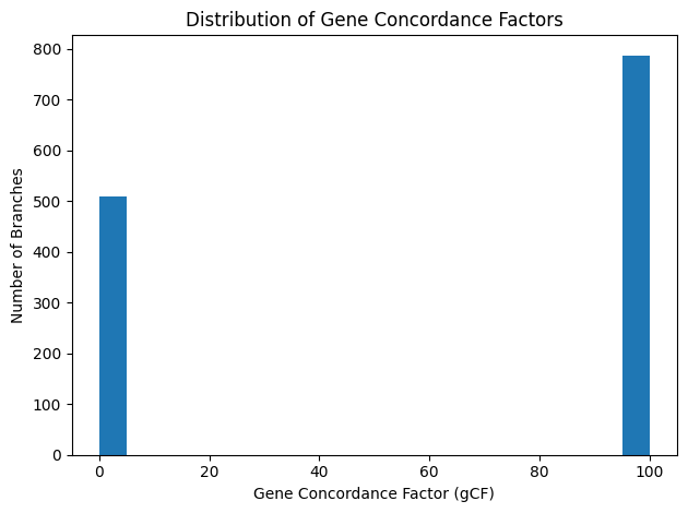
Figure 11: Bar chart of gCF values
The gene concordance factor (gCF) distribution across our ML phylogram is bimodal: with only three loci, each internal branch is either supported by
all three gene trees (gCF = 100%) or by none (gCF = 0%). In fact, 508 branches exhibit gCF = 0%, while 787 branches reach gCF = 100%. This pattern indicates
that no internal split is recovered by more than one marker, meaning that every observed gene‐tree conflict is locus‑specific.
Site concordance factors (sCF) computed on the concatenated alignment provide a much more nuanced view of branch support than gCF. A histogram of likelihood‑based
sCF (Figure 12) reveals that the vast majority of branches carry very little site support—with a clear mode in the 0–5% range—while only a small minority (≈ 5%)
achieve sCF values above 50%. To visualize this, the cumulative distribution function (CDF; Figure 13) plots the fraction of branches exceeding any given sCF
threshold—for example, only about 20% of branches reach 20% or higher site support.
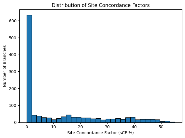
Figure 12: Histogram of likelihood‑based sCF
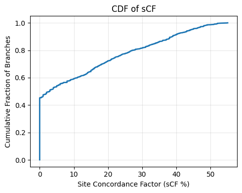
Figure 13: CDF of sCF
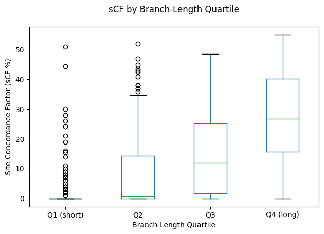
Figure 14: Boxplots of sCF by branch‑length quartile
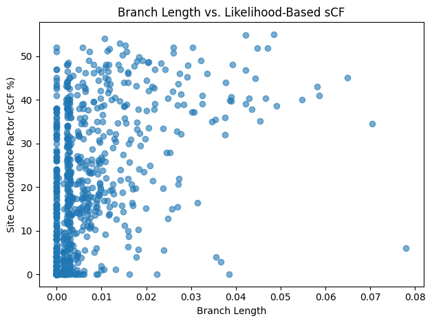
Figure 15: Scatter of branch length vs sCF
We also find that branch length correlates with site concordance. When branches are grouped into quartiles by their length, the shortest 25% of edges have median
sCF near 0%, whereas the longest 25% enjoy a median sCF of roughly 27% (Figure 14). A scatterplot of branch length against sCF (Figure 15) further underscores this
relationship, showing that deeper splits generally accumulate more informative sites.
Finally, counting the number of low‑support branches (Figure 16) highlights that approximately 950 branches fall below 20% sCF, about 1 300 fall below 50%, and
nearly 1 350 fall below 80%. Taken together, these results indicate that although a handful of deep backbone splits are strongly supported by site‑based signal,
the majority of internal branches in our concatenated dataset remain poorly resolved, reflecting the limited phylogenetic information in these three loci for
finer‐scale relationships
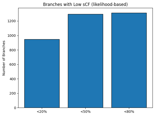
Figure 16: Bar chart of low‑support thresholds (< 20%, < 50%, < 80%)
We did not compute concordance factors on the BEAST MCC tree itself, but our gCF and sCF analyses on the ML phylogram identified a small set of deep, long‑branch splits with strong multi‑locus and site support. The BEAST MCC tree—by enforcing an ultrametric clock and applying birth–death priors - produces a more balanced topology (lower Sackin’s and Colless’ indices) despite remaining fully bifurcating. Because these model choices tend to down‑weight poorly supported shallow splits in the MCMC posterior, the MCC backbone is expected to preserve the robust deep splits highlighted by our CF analysis. This is a confirmation that the BEAST MCC tree is a better choice for our molecular backbone for downstream comparisons.
Implications and challenges
The rDNA backbone will be used to compare the molecular tree with the deep‑learning trees. The close agreement between our BEAST MCC tree and neutral‐coalescent expectations (normalized Colless ≈ 0.25; Sackin deviation within ±1 125) suggests that our dataset — and the birth–death dating prior — effectively compensates for missing lineages and weakly supported splits, yielding a phylogeny whose imbalance reflects real diversification patterns rather than analytical artifacts [1, 2]. Finally, by using this molecular scaffold as the benchmark for CNN‑derived shell‑morphology trees, we can rigorously test whether image‑based models recover genuine evolutionary signal or instead overfit to non‑phylogenetic traits, opening the door to automated, morphology‑informed insights into gastropod macroevolution.
This analysis remains subject to several constraints. (1) Marker choice: rDNA loci evolve at different rates and may not capture very recent radiations or deep splits uniformly; reliance on concatenation could mask locus‑specific conflicts [5, 6]. (2) Taxon sampling: although we mined every public entry, the uneven availability of 28S sequences (92 vs. 661 12S) means some genera remain under‑represented, potentially biasing branch‐length estimates and downstream CNN comparisons. (3) Alignment and trimming: automated gap removal (>90 % threshold) can inadvertently discard informative indels or retain misaligned regions, especially in variable loops of mitochondrial rRNAs. (4) Model assumptions: the use of a single GTR + Γ + I model across concatenated loci assumes homogeneous substitution dynamics; mixed‐model approaches might better accommodate locus‐specific patterns. Acknowledging these limits will guide careful interpretation of any concordance (or discordance) between molecular and image‑derived phylogenies.
Next steps
- creation of a multilocus species tree
- CNN Models for each genus and the family
- Compare the morphological CNN tree with the molecular tree
References
- [1] Goh G, Fuchs M, Zhang L. Two results about the Sackin and Colless indices for phylogenetic trees and their shapes.. J Math Biol. 85(6-7):69 (2022)
- [2] M. J. Sackin. “Good” and “Bad” Phenograms. Systematic Biology, Volume 21, Issue 2, Pages 225–226 (1972)
- [3] Suchard MA et al. Bayesian phylogenetic and phylodynamic data integration using BEAST 1.10. Virus Evolution 4 (2018)
- [4] Cock PA et al. Biopython: freely available Python tools for computational molecular biology and bioinformatics. Bioinformatics, 25, 1422-1423 (2009)
- [5] M Holford et al. Evolution of the Toxoglossa Venom Apparatus as Inferred by Molecular Phylogeny of the Terebridae. Mol. Biol. Evol. 26(1):15–25. (2009)
- [6] Modica, M. V., Gorson, J., Fedosov, A. E., et al. Macroevolutionary analyses suggest that environmental factors, not venom apparatus, play key role in Terebridae marine snail diversification. Systematic Biology 69 (3): 413–430 (2020)
Appendix
Table I. Sequences removed from the 12S Dataset
| Accession | Species | |
|---|---|---|
| EU685366.1 | Punctoterebra fuscotaeniata | |
| EU685455.1 | Profunditerebra poppei | |
| EU685368.1 | Profunditerebra poppei | |
| EU685362.1 | Punctoterebra fuscotaeniata | |
| MK587060.1 | Profunditerebra poppei | |
| EU685464.1 | Punctoterebra succincta | |
| EU685378.1 | Punctoterebra succincta | |
| EU685381.1 | Punctoterebra succincta | |
| EU685372.1 | Punctoterebra succincta | |
| JQ808689.1 | Punctoterebra succincta | |
| MK587109.1 | Myurellopsis nathaliae | |
| MK586849.1 | Terebra guttata | |
| MN657707.1 | Punctoterebra nitida | |
| MN657645.1 | Punctoterebra nitida | |
| MK587153.1 | Punctoterebra nitida | |
| MK586909.1 | Punctoterebra nitida | |
| MK586926.1 | Punctoterebra nitida |
Table II. Sequences removed from the 16S Dataset
| Accession | Species | |
|---|---|---|
| EU685654.1 | Punctoterebra fuscotaeniata | |
| EU685658.1 | Punctoterebra fuscotaeniata | |
| JQ808905.1 | Punctoterebra succincta | |
| EU685757.1 | Punctoterebra succincta | |
| EU685669.1 | Punctoterebra succincta | |
| EU685672.1 | Punctoterebra succincta | |
| MK586365.1 | Hastula lanceata | |
| MN657833.1 | Punctoterebra souleyeti | |
| MK586628.1 | Profunditerebra poppei | |
| EU685748.1 | Profunditerebra poppei | |
| EU685660.1 | Profunditerebra poppei |

Figure 1: 12S rDNA Gene Phylogenetic tree for Terebridae (ML)

Figure 2: 12S rDNA Gene Phylogenetic tree for Terebridae (ML)
_beast.svg)
Figure 3: 12S rDNA Gene Phylogenetic tree for Terebridae (BA)
import msprime, numpy as np
from Bio import Phylo
from io import StringIO

def count_leaves(clade):
    """Recursively count the number of leaves under this clade."""
    if clade.is_terminal():
        return 1
    return sum(count_leaves(child) for child in clade.clades)

def colless_index(tree):
    """
    Colless' index: sum over internal nodes with exactly two children of
    |#leaves(left) - #leaves(right)|.
    """
    idx = 0
    for node in tree.get_nonterminals():
        if len(node.clades) == 2:
            l, r = node.clades
            idx += abs(count_leaves(l) - count_leaves(r))
    return idx

def sackin_index(tree):
    """
    Sackin's index: sum of the depths (number of edges from the root) of all leaves.
    """
    def depth(target, node, d=0):
        if node is target:
            return d
        for child in node.clades:
            dd = depth(target, child, d+1)
            if dd is not None:
                return dd
        return None

    return sum(depth(leaf, tree.root) for leaf in tree.get_terminals())

def expected_sackin(n):
    """Expected Sackin index under Yule: 2 n (H_n - 1)."""
    Hn = sum(1.0/k for k in range(1, n+1))
    return 2 * n * (Hn - 1)

def simulate_coalescent_indexes(n, reps=200):
    colless_vals = []
    sackin_vals = []
    for _ in range(reps):
        # simulate a neutral genealogy of n samples
        tree_seq = msprime.simulate(sample_size=n, Ne=1e5, length=1, recombination_rate=0)
        ts = tree_seq.first()  # take the (only) tree
        newick = ts.as_newick()  # get Newick string
        tree = Phylo.read(StringIO(newick), "newick")

        # compute indices
        C = colless_index(tree)
        S = sackin_index(tree)

        colless_vals.append(C / (n**1.5))
        sackin_vals.append(S - expected_sackin(n))
    return np.array(colless_vals), np.array(sackin_vals)

# Example for 12S tree n = 644
C_coal, S_coal = simulate_coalescent_indexes(644, reps=200)
print("Coalescent null Colless:", np.mean(C_coal), "±", np.std(C_coal))
print("Coalescent null Sackin dev:", np.mean(S_coal), "±", np.std(S_coal))
Figure 4: Python code used for simulation

Figure 5: 16S rDNA Gene Phylogenetic tree for Terebridae (ML)

Figure 6: 16S rDNA Gene Phylogenetic tree for Terebridae (ML)

Figure 7: 16S rDNA Gene Phylogenetic tree for Terebridae (BA)

Figure 8: 28S rDNA Gene Phylogenetic tree for Terebridae (ML)

Figure 9: 28S rDNA Gene Phylogenetic tree for Terebridae (ML)

Figure 10: 28S rDNA Gene Phylogenetic tree for Terebridae (BA)